myXCLASSFit with non-LTE
The purpose of this tutorial is to describe how to model the contribution of a molecule in Non-LTE, see Sect. “Non-LTE description of molecules” using the myXCLASSFit function, see Sect. “myXCLASSFit”.
All files used within this tutorial can be downloaded here.
Introduction
Here, we want to model the contribution of CH\(_3\) OH\(_{v=0}\) A and take the contribution of CH\(_3\) OH\(_{v=0}\) E into account as well. We use observational data of the LMC.
Observational xml file
For the myXCLASSFit function we have to define the frequency range, (here from 241.45 to 241.75 GHz), the size of the interferometric beam (here 0.14 arcsec), the background and dust parameters, respectively.
Observational xml file tutorial-nlte__obs__LMC.xml used for the
myXCLASSFit function:
<?xml version="1.0" encoding="UTF-8"?>
<ExpFiles>


   <!-- define number of observation files -->
   <NumberExpFiles>1</NumberExpFiles>


   <!-- ********************************************************************** -->
   <!-- define parameters for 1st observation data file -->
   <file>


      <!-- define path and name of first data file -->
      <FileNamesExpFiles>files/data/CH3OH_WS_px_1050_1039.dat</FileNamesExpFiles>


      <!-- define import filter -->
      <ImportFilter>xclassASCII</ImportFilter>


      <!-- define number of data ranges -->
      <NumberExpRanges>1</NumberExpRanges>


      <!-- define parameters for each data ranges -->
      <FrequencyRange>
            <MinExpRange>2.414511573992605845e+05</MinExpRange>
            <MaxExpRange>2.417543671618033550e+05</MaxExpRange>
            <StepFrequency>1.2128390501893591</StepFrequency>


            <!-- define background temperature and temperature slope -->
            <t_back_flag>True</t_back_flag>
            <BackgroundTemperature>0.0</BackgroundTemperature>
            <TemperatureSlope>0.0</TemperatureSlope>


            <!-- define hydrogen column density, beta for dust, and kappa -->
            <HydrogenColumnDensity>1.4e+19</HydrogenColumnDensity>
            <DustBeta>1.4</DustBeta>
            <Kappa>0.4</Kappa>
      </FrequencyRange>


      <!-- define size of telescope -->
      <TelescopeSize>0.14</TelescopeSize>


      <!-- define if interferometric observation is modeled -->
      <Inter_Flag>True</Inter_Flag>


      <!-- define local standard of rest (vLSR) -->
      <GlobalvLSR>233.0</GlobalvLSR>


      <!-- define parameters for ASCII file import -->
      <ErrorY>no</ErrorY>
      <NumberHeaderLines>0</NumberHeaderLines>
      <SeparatorColumns> </SeparatorColumns>
   </file>


   <!-- *********************************** -->
   <!-- taken local-overlap into account? -->
   <LocalOverlap_Flag>False</LocalOverlap_Flag>


   <!-- *************************************************************** -->
   <!-- parameters for isotopologues -->
   <iso_flag>True</iso_flag>
   <IsoTableFileName>files/tutorial-nlte__iso-ratios.dat</IsoTableFileName>


   <!-- *************************************************************************************** -->
   <!-- define file describing collision partners -->
   <CollisionPartnerFileName>files/tutorial-nlte__collision-partners.dat</CollisionPartnerFileName>
</ExpFiles>
In contrast to the LTE description, the Non-LTE description requires
the collision rates for the corresponding molecules and the density of
the collision partners, which are described in the collision partner
file, see Sect. “The collision partner file”. In the aforementioned obs.
xml file, the path and name of this collision partner file is described
by tag <CollisionPartnerFileName>.
Molfit file
Methanol is the simplest asymmetric-top molecule with one hindered torsion and eleven normal vibration modes. The rotational and vibration-rotational spectra of methanol are complicated by various interactions among torsion, rotation, and vibrations, which have been extensively studied for many years in microwave, far-infrared, and infrared frequency regions.
It has a symmetric group and a locally rotated axis (i.e., CH\(_3\) axis) of symmetry, it rotates around this methyl group axis with internal rotation or torsion of the CH\(_3\) group relative to the OH group. The identical nuclei in the CH\(_3\) group give rise to the existence of a specific type of nuclear spin isomers in methanol. It is from the three spin-1/2 hydrogen nuclei of the CH\(_3\) group that the ortho-CH\(_3\)OH (I = 3/2) and para-CH\(_3\)OH (I = 1/2) are formed in methanol, which are distinguished respectively by the symmetry quantum numbers \(\sigma\) = 0 and ± 1. The ortho-CH\(_3\)OH isomer corresponds to the symmetry quantum number \(\sigma\)= 0. Accordingly for the para-CH\(_3\)OH isomer to \(\sigma\)= ±1. Here each \(\sigma\)value corresponds to a torsional-symmetry species of A-species (\(\sigma\)= 0, CH\(_3\)OH\(_{v=0}\) A) and E-species (\(\sigma\)= ±1, CH\(_3\)OH\(_{v=0}\) E).
The relative abundance of the ortho and para nuclear spin isomers in astrophysical environments can provide insights into the temperature and physical conditions of the observed sources. Ortho-methanol is the more abundant nuclear spin isomer at low temperatures due to its lower energy state. Para-methanol is the more abundant nuclear spin isomer at high temperatures due to its higher energy state.
In order to describe a component of a certain molecule in Non-LTE, the
keyword Non-LTE has to be added on the right side of the column
describing the ordering (distance) parameter of the corresponding
component.
The molfit file tutorial-non-lte__Band_6.molfit used for the
myXCLASSFit function:
%=======================================================================================================================================================================================================================================================================
%
% define database parameters:
%
%=======================================================================================================================================================================================================================================================================
%%MinNumTransitionsSQL = 1                % (min. number of transitions)
%%MaxNumTransitionsSQL = 90000            % (max. number of transitions)
%%MaxElowSQL = 8.000e+03                  % (max. lower energy, i.e. upper limit of the lower energy of a transition)
%%MingASQL = 1.000e-09                    % (minimal intensity, i.e. lower limit of gA of a transition)
%%TransOrderSQL = 1                       % (order of transitions: (=1): by lower energy, (=2) by gA, (=3) gA/E_low^2, else trans. freq.)


%=======================================================================================================================================================================================================================================================================
%
% define molecules and their components:
%
%=======================================================================================================================================================================================================================================================================
CH3OH;v=0;A   1
            n        1.00     1000.00         500.00000    y       10.00      200.00          30.00000    y    1.00e+12    1.00e+21       8.00000e+15    y        0.10        9.00           2.00000    y     -250.00      100.00           0.00000   c      Non-LTE
Iso ratio file
Here, the iso ratio file is used to describe the ratio between CH\(_3\)OH\(_{v=0}\) A and CH\(_3\)OH\(_{v=0}\) E.
The iso-ratio file tutorial-nlte__iso-ratios.dat used for the
myXCLASSFit function:
% Isotopologue:      Iso-master:        Iso-ratio:      Lower-limit:      Upper-limit:       collision rate file:
CH3OH;v=0;E          CH3OH;v=0;A               1.0               1.0               1.0       files/e-ch3oh.dat
Here, the last column describes the path and name of the file describing the collision rates of CH\(_3\)OH\(_{v=0}\) E.
Collision partner file
The collision partner file is used, among other things, to describe the name and density of the collision partners, see Sect. “The collision partner file”.
The collision partner file tutorial-nlte__collision-partners.dat used
for the myXCLASSFit function:
%---------------------------------------------------------------------------------------------------------------------------------------------------------
%
% input file for collision partners
%
% densities can be fitted by declaring lower and upper limits, if both limits
% are identical, corresponding density is not fitted.
%
% comments are marked with "%" sign
%
%
%---------------------------------------------------------------------------------------------------------------------------------------------------------
1                                                                                       % Geometry (=1: sphere, =2: LVG, =3: slab)
1                                                                                       % number of molecules
CH3OH;v=0;A                                                                             % molecule
files/tutorial-nlte__coll-rates__a-ch3oh.dat                                            % path and name of file containing collision rates
1                                                                                       % number of collision partners
H2                                                                                      % first collision partner
5.2E+03            1.e2            5.e5                                                 % density of first collision partner
Here, the initial density of the collision partner H\(_2\) is set to \(5.2 \cdot 10^{3}\) cm\(^{-3}\).
Algorithm xml file
In order to fit the parameters described in the molfit, iso ratio, and collision
partner files, we have to define the optimization algorithm(s) which is (are)
used by the myXCLASSFit function. Here, we use the trf algorithm, where we
want to limit the number of iterations to 10 by using the tag
"<number_iterations>". Furthermore, we define another stopping criterion
by setting tag the upper limit of the \(\chi^2\) function to
\(1 \cdot 10^{-15}\), using the tag "<limit_of_chi2>". Additionally, we
want to use 14 processors cores, which is described by tag "<NumberProcessors>".
Algorithm xml file tutorial-nlte__algorithm.xml used for the
myXCLASSFit function:
<?xml version="1.0" encoding="UTF-8"?>
<FitControl>
   <!-- settings for fit process -->


   <!-- set number of used algorithms -->
   <NumberOfFitAlgorithms>1</NumberOfFitAlgorithms>


   <!-- define algorithm -->
   <algorithm>
      <FitAlgorithm>trf</FitAlgorithm>


      <!-- define value of the variation -->
      <VariationValue>1.e-4</VariationValue>


      <!-- set max. number of iterations -->
      <number_iterations>10</number_iterations>


      <!-- set max. number of processors -->
      <NumberProcessors>14</NumberProcessors>


      <!-- set path and name of host file -->
      <MPIHostFileName> </MPIHostFileName>


      <!-- settings for chi^2 -->
      <limit_of_chi2>1e-15</limit_of_chi2>
      <RenormalizedChi2>yes</RenormalizedChi2>
      <DeterminationChi2>default</DeterminationChi2>
      <SaveChi2>yes</SaveChi2>


      <!-- set plot options -->
      <PlotAxisX>Rest Frequency [MHz]</PlotAxisX>
      <PlotAxisY>T_mb [K]</PlotAxisY>
      <PlotIteration>no</PlotIteration>
   </algorithm>
</FitControl>
Call of myXCLASSFit function
Now everything is prepared to start the myXCLASSFit function.
Start myXCLASSFit function
>>> from xclass import task_myXCLASSFit
>>> import os

## get path of current directory
>>> LocalPath = os.getcwd() + "/"

# import XCLASS packages
>>> from xclass import task_myXCLASSFit

# define path and name of molfit file
>>> MolfitsFileName = LocalPath + "files/tutorial-nlte__LMC.molfit"

# define path and name of obs. xml file
>>> ObsXMLFileName = LocalPath + "files/tutorial-nlte__obs__LMC.xml"

# define path and name of algorithm xml file
>>> AlgorithmXMLFileName = LocalPath + "files/tutorial-nlte__algorithm.xml"

# set optimization package
>>> Optimizer = "scipy"

# define if results of myXCLASSFit function are return as dictionary
>>> DictOutFlag = True

# call myXCLASSFit function
>>> OutputDictionary = task_myXCLASSFit.myXCLASSFitCore( \
                             MolfitsFileName = MolfitsFileName, \
                             AlgorithmXMLFileName = AlgorithmXMLFileName, \
                             ObsXMLFileName = ObsXMLFileName, \
                             Optimizer = Optimizer, \
                             DictOutFlag = DictOutFlag)
Results
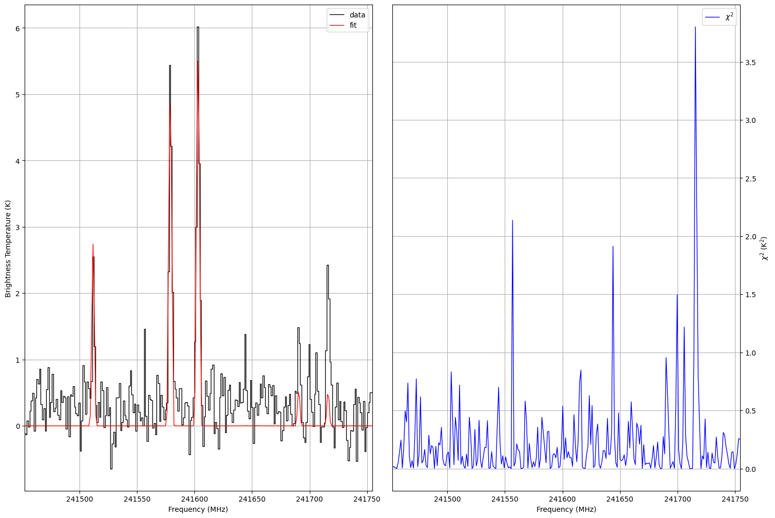
Fig. 25 Fitted spectrum (left panel) and corresponding \(\chi^2\) function (right panel) created by the myXCLASSFit function.
After finishing we get the following molfit file
%=========================================================================================================================================================
%
% define database parameters:
%
%=========================================================================================================================================================
%%MinNumTransitionsSQL = 1                % (min. number of transitions)
%%MaxNumTransitionsSQL = 90000            % (max. number of transitions)
%%MaxElowSQL = 8.000e+03                  % (max. lower energy, i.e. upper limit of the lower energy of a transition)
%%MingASQL = 1.000e-09                    % (minimal intensity, i.e. lower limit of gA of a transition)
%%TransOrderSQL = 1                       % (order of transitions: (=1): by Elow, (=2) by gA, (=3) gA/E_low^2, else trans. freq.)


%=========================================================================================================================================================
%
% define molecules and their components:
%
%=========================================================================================================================================================
CH3OH;v=0;A  1
   n        1.00     1000.00         500.00000    y       10.00      200.00          11.49368    y    1.00e+12    1.00e+21       9.90429e+15    y        0.10        9.00           1.96329    y     -250.00      100.00           0.62725      c      Non-LTE
Additionally, we get an density of \(8.53 \cdot 10^{4}\) cm\(^{-3}\) for the collision partner H\(_2\).