CubeFit

The purpose of this tutorial is to describe the usage of the CubeFit function, see Sect. “CubeFit”, to fit model parameters of a physical model to a given data cubes.

All files used within this tutorial can be downloaded here.

Observational xml file

For the CubeFit function we have to define the frequency range, (here from 348.863 to 349.561 GHz), the size of the interferometric beam (here 0.37 arcsec), the background and dust parameters. Here, we use a synthetic data cube, where we know, which model parameters were used.

Observational xml file tutorial-cubefit__obs.xml used for the CubeFit function:

<?xml version="1.0" encoding="UTF-8"?>
<ExpFiles>


   <!-- define number of experimental data file(s) -->
   <NumberExpFiles>1</NumberExpFiles>


   <!-- ********************************************************************** -->
   <!-- define parameters for FIRST file -->
   <file>


      <!-- define path and name of obs. data file -->
      <FileNamesExpFiles>files/data/Synthetic-Cube__Core.fits</FileNamesExpFiles>


      <!-- define import filter -->
      <ImportFilter>xclassFITS</ImportFilter>


      <!-- define number of frequency ranges for first data file -->
      <NumberExpRanges>1</NumberExpRanges>


      <!-- define parameters for each frequency range -->
      <FrequencyRange>
            <MinExpRange>348863.554844</MinExpRange>
            <MaxExpRange>349561.76393600577</MaxExpRange>
            <StepFrequency>0.6989080000057584</StepFrequency>


            <!-- define background temperature and temperature slope -->
            <t_back_flag>True</t_back_flag>
            <BackgroundTemperature>0.0</BackgroundTemperature>
            <TemperatureSlope>0.0</TemperatureSlope>


            <!-- define hydrogen column density, beta for dust, and kappa -->
            <HydrogenColumnDensity>1.0e+22</HydrogenColumnDensity>
            <DustBeta>2.0</DustBeta>
            <Kappa>0.0</Kappa>
      </FrequencyRange>


      <!-- define local standard of rest (vLSR) -->
      <GlobalvLSR>0.0</GlobalvLSR>


      <!-- define size of telescope -->
      <TelescopeSize>0.37</TelescopeSize>


      <!-- define if interferrometric observation is modeled -->
      <Inter_Flag>True</Inter_Flag>
   </file>


   <!-- ************************************** -->
   <!-- taken local-overlap into account? -->
   <LocalOverlap_Flag>False</LocalOverlap_Flag>-->


   <!-- **************************** -->
   <!-- prevent sub-beam description -->
   <NoSubBeam_Flag>True</NoSubBeam_Flag>


   <!-- ************************************************ -->
   <!-- parameters for isotopologues -->
   <iso_flag>False</iso_flag>
   <IsoTableFileName>files/iso-ratios.dat</IsoTableFileName>
</ExpFiles>

Molfit / model file

Here we do not need a molfit file, but a python function, which generates the input file(s) (molfit, iso ratio, or collision partner file) for a given pixel coordinate. The python function is described by the script core.py located in the subdirectory model.

Iso ratio file

Here, no iso-ratio file is used.

Algorithm xml file

In order to fit the model parameters used in python script core.py, we have to define the optimization algorithm(s) which is (are) used by the CubeFit function. Here, we use the trf algorithm, where we want to limit the number of iterations per pixel to 5 by setting the tag "<number_iterations>" to 5. Furthermore, we define another stopping criterion by setting tag the upper limit of the \(\chi^2\) function to \(1 \cdot 10^{-6}\), using the tag "<limit_of_chi2>". Additionally, we want to use 40 processor cores in parallel, which is described by tag "<NumberProcessors>". Please note, the number of used cores depends on the used optimization algorithm. Here, we use the trf algorithm with five free parameters. Additionally, we fit \(12 \times 9 = 108\) pixels. In total \((5 + 1) \times 108 = 648\) spectra has to be calculated. (Many optimization algorithms compute the gradient of the \(\chi^2\) function for each iteration step. This gradient has five entries plus an additional call for the unmodified parameter vector.)

Algorithm xml file tutorial-cubefit__algorithm__trf.xml used for the CubeFit function:

<?xml version="1.0" encoding="UTF-8"?>
<FitControl>
   <!-- settings for fit process -->


   <!-- set number of used algorithms -->
   <NumberOfFitAlgorithms>1</NumberOfFitAlgorithms>


   <!-- define settings for 1st algorithm -->
   <algorithm>
      <FitAlgorithm>trf</FitAlgorithm>


      <!-- set variation value -->
      <VariationValue>1.e-3</VariationValue>


      <!-- set max. number of iterations -->
      <number_iterations>5</number_iterations>


      <!-- set max. number of processors -->
      <NumberProcessors>40</NumberProcessors>


      <!-- settings for chi^2 -->
      <LimitChi2>1e-6</LimitChi2>
      <RenormalizedChi2>True</RenormalizedChi2>
      <LogChi2>True</LogChi2>
      <SaveChi2>True</SaveChi2>


      <!-- set plot options -->
      <PlotFlag>True</PlotFlag>
   </algorithm>
</FitControl>

Call of CubeFit function

Now everything is prepared to start the CubeFit function.

Start CubeFit function

>>> from xclass import task_CubeFit
>>> import os

## get path of current directory
>>> LocalPath = os.getcwd() + "/"

# import XCLASS packages
>>> from xclass import task_CubeFit

# extend sys.path variable
# the function to calculate the molfit file is outsourced
# to make this script clearer.
# extend sys.path variable
>>> NewPath = LocalPath + "files/model/"
>>> if (not NewPath in sys.path):
>>>     sys.path.append(NewPath)

# import python script containing the model generator
# and the definitions of the parameters
>>> import core

# define path and name of obs. xml file
>>> ObsXMLFileName = LocalPath + "files/tutorial-cubefit__obs.xml"

# define path and name of algorithm xml file
>>> AlgorithmXMLFileName = LocalPath + "files/alg/tutorial-cubefit__algorithm__trf.xml"

# define path and name of ds9 region file
>>> regionFileName = ""

# define path and name of FITS image file describing selected pixels and weights
>>> FITSImageMaskFileName = ""

# define python function, which computes the content of the moflit file
# for a given pixel position
# The function "GenerateInputFiles" is executed by the CubeFit function
# for each selected pixel
>>> CubeFitObj = core.GenerateInputFiles

# define python dictionary, which defines all required model parameters
# used by function "CubeFitObj"
>>> ModelParamDict = core.GenerateParameterDict()

# call CubeFit function
>>> CubeFitReturnVariable = task_CubeFit.CubeFitCore(
                                ObsXMLFileName = ObsXMLFileName, \
                                AlgorithmXMLFileName = AlgorithmXMLFileName, \
                                regionFileName = regionFileName, \
                                FITSImageMaskFileName = FITSImageMaskFileName, \
                                CubeFitObj = CubeFitObj, \
                                CubeFitParamDict = ModelParamDict)

## get results from CubeFit function
# "CubeFitJobDir": describes path and name of job directory
# "CubeFitParamDict": python dictionary with optimized fit parameters
# "CubeFitFitParam": list of fit parameters
>>> JobDir = CubeFitReturnVariable["CubeFitJobDir"]
>>> CubeFitParamDict = CubeFitReturnVariable["CubeFitParamDict"]
>>> CubeFitFitParam = CubeFitReturnVariable["CubeFitFitParam"]

Results

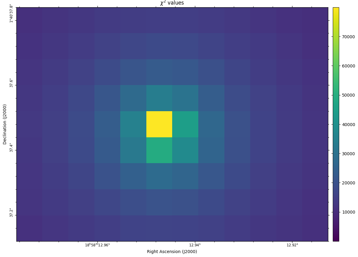
Fig. 35 The \(\chi^2\) values, i.e. the summed squared differences for each pixel.

The CubeFit function creates a FITS image describing the \(\chi^2\) value for each selected pixel. Additionally, a FITS cube is created describing the synthetic spectrum for each selected pixel.