myXCLASS
creating single, synthetic spectra
The myXCLASS function is the core of XCLASS and models a spectrum by solving the radiative transfer equation for an isothermal object in one dimension, called detection equation [Stahler_Palla_2005]. Here, the user can define, if LTE is assumed, i.e. if the source function is given by the Planck function of an excitation temperature [2] or, if a Non-LTE description within the escape probability method is used instead. The myXCLASS function is designed to describe line-rich sources which are often dense, where LTE is a reasonable approximation. Additionally, a Non-LTE description requires collision rates which are available only for a few molecules, see Sect. “Non-LTE description of molecules”. Details of the myXCLASS function are described in Sect. “myXCLASS”.
Example call of the myXCLASS function:
>>> from xclass import task_myXCLASS
>>> import os

# get path of current directory
>>> LocalPath = os.getcwd() + "/"

## define path and name of molfit file
>>> MolfitsFileName = LocalPath + "files/12C.molfit"

## define path and name of obs. xml file
>>> ObsXMLFileName = LocalPath + "files/SMF_obs.xml"

# call myXCLASS function
>>> spectra, log, te, IntOpt, JobDir = task_myXCLASS.myXCLASSCore(MolfitsFileName = MolfitsFileName, \
                                                                  ObsXMLFileName = ObsXMLFileName)
What is myXCLASS?
The myXCLASS function is able to model a spectrum with an arbitrary number of molecules where the contribution of each molecule is described by an arbitrary number of components. These could be identified with clumps, hot dense cores etc. The myXCLASS function offers the possibility to describe the position and shape of each component in a simple 1-d, see Sect. “Simple 1-d description”, or in an advanced 3-d description, see Sect. “Stacking” and Sect. “Sub-beam description”. Additionally, myXCLASS is able to take the local and non-local overlap between different lines into account, see Sect. “Local-overlap of neighboring lines”.
In general, the myXCLASS function assumes, that all components are
aligned in a user-defined stack along the line-of-sight, where the
background and the observer are located at the ends, respectively. The
solution of the radiative transfer equation for components which are
located in a layer (i=1) closest to the background is [3],
where the sums go over the indices \(m\) for molecule, and \(c\) for component, respectively. In the following we will briefly describe each term in Eq. (1).
The beam filling (dilution) factor \(\eta(\theta^{m,c})\) of molecule \(m\) and component \(c\) in Eq. (1) for a source with a Gaussian brightness profile, see below, and a Gaussian beam is given by [4]
where \(\theta^{m,c}\) and \(\theta_t\) represents the source
and telescope beam full width half maximum (FWHM) sizes, respectively.
The sources beam FWHM sizes \(\theta^{m,c}\) (in arcsec) for the different
components are defined by the user in the molfit file, described in
Sect. “The molfit file”. Additionally, the myXCLASS program
assumes for single dish observations (indicated by
Inter_Flag = False), that the telescope beam FWHM size is related to
the diameter of the telescope by the diffraction limit
where \(D\) describes the diameter of the telescope,
\(c_{\rm light}\) the speed of light, and
\(\xi = 3600 \cdot 180 /\pi\) a conversion factor to get the
telescope beam FWHM size in arcsec. For interferometric observations
(indicated by Inter_Flag = True, the user has to define the
interferometric beam FWHM size directly using parameter
TelescopeSize. In contrast to single dish observations the
myXCLASS program assumes a constant interferometric beam FWHM size
for the whole frequency range.
In general, the brightness temperature of radiation temperature \(J(T, \nu)\) is defined as
The expression \(J_\mathrm{CMB}\) describes the radiation temperature Eq. (4) of the cosmic background \(T_{\rm cbg}\) = 2.7 K, i.e. \(J_\mathrm{CMB} \equiv J(T_{\rm cbg}, \nu)\).
In Eq. (1), the expression \(S^{m,c}(\nu)\) represents the source function and is according to Kirchhoff’s law of thermal radiation given by
where \(\epsilon_{i}^{m,c}(\nu)\) and
\(\kappa_{i}^{m,c}(\nu)\) are the emission and absorption
coefficients for line, dust, free-free, and synchrotron, respectively.
Additionally, the optical depth is given by
\(\tau^{m,c}_i(\nu) = \int \kappa^{m,c}_i(\nu) \, ds\), which
assumes that molecules and continuum contributions are well mixed. In
older versions, the background temperature could only be defined as
the measured continuum offset, which corresponds to the beam-averaged
continuum brightness temperature. At the same time, the dust, as agent
of line attenuation, was described by column density and opacity. This
is practical, because the observable \(T_{\rm bg}\) is used, but
does not constitute a self-consistent and fully physical description.
Therefore, we now use optionally either a physical
(\(\gamma \equiv 1\), defined by the input parameter setting
t_back_flag = False) or phenomenological (\(\gamma \equiv 0\),
defined by the input parameter setting t_back_flag = True)
description of the background indicated by the Kronecker delta
\(\delta_{\gamma, 0}\),
i.e. \(S^{m,c}(\nu) \equiv J(T_\mathrm{ex}^{m,c}, \nu)\) for
\(\gamma \equiv 0\). Note, if \(\gamma \equiv 0\), the
definition of the dust temperature \(T_d^{m,c} (\nu)\),
Eq. (33), is superfluous.
The total optical depth \(\tau_{\rm total}^{m,c}(\nu)\) of each molecule \(m\) and component \(c\) is defined as the sum of the optical depths \(\tau_l^{m,c}(\nu)\) of all lines of each molecule \(m\) and component \(c\) plus the dust optical depth \(\tau_{\rm dust}^{m,c}(\nu)\) (see Sect. “Dust contribution”), the free-free optical depth \(\tau_{\rm free-free}^{m,c}(\nu)\) (see Sect. “Free-free contribution”), and the synchrotron optical depth \(\tau_{\rm sync}^{m,c}(\nu)\) (see Sect. “Synchrotron contribution”), i.e.
(6)\[\tau_{\rm total}^{m,c}(\nu) = \tau_l^{m,c}(\nu) + \tau_{\rm dust}^{m,c}(\nu) + \tau_{\rm free-free}^{m,c}(\nu) + \tau_{\rm sync}^{m,c}(\nu)\]
The optical depth \(\tau_t^{m,c}(\nu)\) for a transition \(t\) of molecule \(m\) and component \(c\) is described as [5]
where \(\phi^{m,c,t}(\nu)\) indicates a line profile function, described in Sect. “Line profile function”. The Einstein \(A_{ul}\) coefficient [6], the energy of the lower state \(E_l\), the upper state degeneracy \(g_u\), and the partition function [7] \(Q \left(m, T_{\rm ex}^{m,c} \right)\) of molecule \(m\) are taken from the embedded SQLite3 database. In addition, the values of the excitation temperatures \(T_{\rm ex}^{m,c}\) and the column densities \(N_{\rm tot}^{m,c}\) for the different components and molecules are taken from the user defined molfit file.
If local-overlap of lines is not taken into account
(LocalOverlapFlag = False) the optical depth
\(\tau_l^{m,c}(\nu)\) of all lines for each molecule \(m\) and
component \(c\) is described as
where the sum with index \(t\) runs over all spectral line transitions of molecule \(m\) within the given frequency range. The calculation procedure including local-overlap is described in Sect. “Local-overlap of neighboring lines”.
The beam-averaged continuum background temperature \(I_{\rm bg} (\nu)\) is parameterized as
to allow the user to define the continuum contribution for each frequency range, individually. Here, \(\nu_{\rm min}\) indicates the lowest frequency of a given frequency range. \(T_{\rm bg}\) and \(T_{\rm slope}\), defined by the user, describe the background continuum temperature and the temperature slope, respectively. Additionally, XCLASS offers the possibility to describe the background continuum, i.e. the continuum seen by the layer close to the cosmic microwave background, by a so-called background file \(I_{\rm bg}^{\rm file} (\nu)\).
Finally, the last term \(J_\mathrm{CMB}\) in
Eq. (1) describes the OFF position for
single dish observations (defined by Inter_Flag = False) where
we have an intensity caused by the cosmic background
\(J_\mathrm{CMB}\). For interferometric observations, the
contribution of the cosmic background is filtered out and has to
be subtracted as well.
Hence, the layers, which do not belong to the largest distance parameter, have to be considered in an iterative manner where the solution of the radiative transfer equation for a certain distance \(i>1\) can be expressed as
where \(m\) and \(c\) indicates the index of the current molecule and component, respectively. Here, the expression \(T_{\rm mb}^{\rm i=1}(\nu)\), described by Eq. (1), represents the spectrum caused by layers which are closest to the background, including the beam-averaged continuum background temperature \(I_{\rm bg}^{\rm core} (\nu)\). The contribution by other components (\(i > 1\)) is considered by first calculating \(T_{\rm mb}^{\rm i=1}(\nu)\) and then use this as new continuum for lines at distance \(i\).
By fitting all species and their components at once, line blending and optical depth effects are taken into account. The modeling can be done simultaneously with isotopologues (and higher vibrational states) of a molecule assuming an isotopic ratio stored in the so-called iso ratio file, see Sect. “The iso ratio file”. Here, all parameters are expected to be the same except the column density which is scaled by one over the isotopic ratio for each isotopologue. Additionally, it is assumed that radiation emitted by all isotopologues of a molecule in a component interact with all other isotopologues, but the radiation emitted in one component does not interact with other molecules or with the same molecule in different components, i.e. their intensities are added, except local-overlap is taken into account, see Sect. “Local-overlap of neighboring lines”.
In order to correctly take instrumental resolution effects into account in comparing the modeled spectrum with observations, myXCLASS integrates the calculated spectrum over each channel. Thereby, myXCLASS assumes that the given frequencies \(\nu\) describe the center of each channel, respectively. The resulting value is than given as
(10)\[T_{\rm mb}(\nu) = \frac{1}{\Delta_c} \int_{\nu-\frac{\Delta_c}{2}}^{\nu+\frac{\Delta_c}{2}} T_{\rm mb}(\tilde{\nu}) d\tilde{\nu},\]
where \(\Delta_c\) represents the width of a channel. Due to the complexity of Eqn. (1), (9) the integration in Eq. (10) can not be done analytically. Therefore, myXCLASS performs a piecewise integration of each component and channel using the trapezoidal rule and summaries the resulting values to get the final value used in Eq. (10). In order to reduce the computation effort myXCLASS determines the minimal line width of all components of a certain distance. If a channel contains no transition, myXCLASS determines the intensities at \(\nu \pm \frac{\Delta_c}{2}\) and evaluates Eq. (10) by applying the trapezoidal rule. But, if transitions are included, myXCLASS re-samples the corresponding channel, whereby the number \(n_\nu\) of additional frequency points is given by
\[n_\nu = (m \cdot 3) \cdot \min \left[1, {\rm int} \left[\frac{\Delta_c}{\sigma_{\rm min}} \right] \right],\]
where \(m\) represents the number of transitions contained in the current channel and \(\sigma_{\rm min} = \frac{\Delta v_{\rm min}}{2 \, \sqrt{2 \, \ln \, 2} \, c_{\rm light}} \, \nu\). If local-overlap is taken into account, see Sect. “Local-overlap of neighboring lines”, \(\Delta v_{\rm min}\) indicates the minimal line width of all components of the current layer, otherwise \(\Delta v_{\rm min}\) describes the line width of the current component. Here, the function int(\(x\)) gives the integer part of \(x\). Finally, myXCLASS computes the intensities at these frequencies and evaluates Eq. (10).
The molfit file
Within the molfit file the user defines both which molecules (or radio recombination lines (RRLs), continuum contributions) are taken into account and how many components are used. The definition of parameters for a molecule (or RRLs, continuum contributions) starts with a line describing the name of the molecule [8] (or RRLs, continuum contributions), followed by the number of components \(N\). The following \(N\) lines describe the parameters for each components, separately. The number of columns and their meaning depends on the modeled contribution (molecule, RRL, or continuum contribution). Generally, all parameters have to be separated by blanks, comments are marked with the % character.
Molecules
For molecules, the user has to define for each component the excitation
temperature \(T_{\rm ex}\) in K (T_rot), the column density
\(N_{\rm tot}\) in cm\(^{-2}\) (N_tot), and the velocity
offset (relative to v\(_{\rm LSR}\)) in km s\(^{-1}\)
(V_off). Depending of the used source description, see
Sect. “Source description”, the size of the source
\(\theta^{m,c}\) in arcsec (s_size) and their offset relative to
the beam center is required as well. Furthermore, the selected line
profile requires one or two velocity widths (FWHM) \(\Delta \nu\) in
km s\(^{-1}\) (V_width). Additionally, the stacking of the
components along the line-of-sight requires the cf-flag (CFFlag),
see Sect. “Simple 1-d description”, or the distance parameter
(distance), see Sect. “Stacking”. Finally,
the column (keyword) to describe so-called keywords, indicating the
line profile function, Non-LTE description etc. Note, different keywords
have to be separated by “_” character. For example, the composed
keyword Non-LTE_Voigt indicates a Non-LTE description and the usage
of a Voigt line profile for the corresponding component.
Example of a molfit file describing two molecules CS\(_{v=0}\) and HCS\(^+_{v=0}\) with two components, respectively:
% Number of molecules = 2
% s_size:  T_rot:    N_tot:  V_width:   V_off:  CFFlag:   keyword:
CS;v=0;   3
   48.470  300.00  3.91E+17      2.86  -20.564        c
   21.804  320.00  6.96E+17      8.07   30.687        c
   81.700  208.00  1.46E+17      5.16  -10.124        c
HCS+;v=0;   2
% s_size:  T_rot:    N_tot:  V_width:   V_off:  CFFlag:   keyword:
           150.00  1.10E+18      5.00   -0.154        f
           200.00  2.20E+17      3.10   -2.154        f
Limiting the number of transitions
XCLASS offers the possibility to limit the number of transitions of molecules which enter Eq. (1). Therefore, the user has to add the following command words to the beginning of the molfit file:
"%%MinNumTransitionsSQL": defines the minimum number of transitions, i.e. XCLASS takes only those molecules into account which have at least this number of transition in the given frequency ranges."%%MaxNumTransitionsSQL"describes the max. number of transitions (in conjunction with"%%TransOrderSQL"). Here,"0"means all transitions are included."%%TransOrderSQL"(in conjunction with"%%MaxNumTransitionsSQL") defines the order of transition. (E.g."%%MaxNumTransitionsSQL = 10"and"%%TransOrderSQL = 1"means, that only the first 10 transitions with the lowest lower energy are taken into account.)"%%MaxElowSQL"defines the upper limit of the lower energy of a transition."%%MingASQL"describes the lower limit of gA (upper state degeneracy * Einstein A coefficient) of a transition.
"%%MinNumTransitionsSQL" and "%%MaxNumTransitionsSQL" are
taken into account.%==============================================================================
%
% define transition parameters:
%
%==============================================================================
%%MinNumTransitionsSQL = 1 % min. number of transitions
%%MaxNumTransitionsSQL = 0 % max. number of transitions,
% =0): all transitions are taken into account
%%TransOrderSQL = 1 % order of transitions:
% (=1): by lower energy,
% (=2): by gA,
% (=3): gA/E_low^2, else by trans. freq.
%%MaxElowSQL = 1.0e+06 % max. lower energy, i.e. upper limit of
% the lower energy of a transition
%%MingASQL = 0.0 % minimal intensity, i.e. lower limit of
% gA of a transition
%==============================================================================
%
% define molecules and their components:
%
%==============================================================================
% s_size: T_rot: N_tot: V_width: V_off: CFFlag: keyword:
CS;v=0; 3
48.470 300.00 3.91E+17 2.86 -20.564 c
21.804 320.00 6.96E+17 8.07 30.687 c
81.700 208.00 1.46E+17 5.16 -10.124 c
HCS+;v=0; 2
% s_size: T_rot: N_tot: V_width: V_off: CFFlag: keyword:
150.00 1.10E+18 5.00 -0.154 f
200.00 2.20E+17 3.10 -2.154 f
The iso ratio file
In order to reduce the number of model parameters, XCLASS offers the
possibility to use a so-called iso ratio file. Here, XCLASS assumes,
that both molecules (isotopologue and iso master molecule) are described
by the same number of components, where the source size, the rotation
temperature, the line width, and the velocity offset are identical. The
corresponding column densities of the isotopologue
\(\left({\rm N}_{\rm tot}^{\rm (isotopologue)}\right)\) are scaled
by the so-called iso ratio, i.e.
The iso ratio file contains three columns separated by tabs or at
least two blank characters, where the first two columns indicates the
isotopologue and the corresponding iso master molecule, respectively.
The third column defines the ratio for both molecules. Comments are
marked with a % character, i.e. all characters on the right side of
a % are ignored.
Example for an iso ratio file:
% isotopologue:         molecule:        ratio:
HC-33-S+;v=0;           HCS+;v=0;          75.0
HC-34-S+;v=0;           HCS+;v=0;          22.5
CS;v=4;                 CS;v=0;             2.3
CS;v=3;                 CS;v=0;             2.1
CS;v=2;                 CS;v=0;             2.1
CS;v=1;                 CS;v=0;             2.0
CS-34;v=0;              CS;v=0;            22.5
CS-34;v=1;              CS;v=0;            22.5
CS-33;v=1;              CS;v=0;            75.0
CS-33;v=0;              CS;v=0;            75.0
In the example described above we define in the first line an iso ratio
of 75.0 between HC-33-S+;v=0; and HCS+;v=0;. Assuming that
HCS+;v=0; is described with one component and with a column density
of \(9 \cdot 10^{16}\) cm\(^{-2}\) the column density of
HC-33-S+;v=0; is
Globally defined iso-ratios
In addition, the user can defined so-called globally defined iso ratios, e.g. (\(^{12}\)C / \(^{13}\)C). This defined ratio is multiplied to all ratios of isotopologues in the iso ratio file which contain e.g. \(^{13}\)C raised to the power of occurrences of the globally defined ion in each isotopologue. For example, the ratio (\(^{12}\)C / \(^{13}\)C) is set globally to 45. Additionally, we set the ratio of (CH\(_3\)CN,v=0 / \(^{13}\)CH\(_3 ^{13}\)CN,v=0) to 3.0. The final iso ratio used by XCLASS for (CH\(_3\)CN,v=0 / \(^{13}\)CH\(_3 ^{13}\)CN,v=0) is then given by \(3.0 \times 45^2 = 6075\). (Here, the exponent \(2\) is caused by the two \(^{13}\)C ions). Additionally, globally defined iso-ratios can be combined as well. In order to determine the used iso ratio for e.g. (\(^{12}\)C\(^{32}\)S)/(\(^{13}\)C \(^{33}\)S) we just have to multiply the globally defined is ratios for (\(^{12}\)C / \(^{13}\)C) and (\(^{32}\)S / \(^{33}\)S).
Globally defined ratios in the iso ratio file are indicated by the
phrase “GLOBAL__” and can not be used alone without other iso
ratios, e.g.
% isotopologue:         molecule:           ratio:
GLOBAL__C-13            C-12                45.0
HO-18;v=0;              OH;v=0;             500
HDO-18;v=0;             HDO;v=0;            500
C-13-H3C-13-N;v=0;      CH3CN;v=0;          1.0
Fitting iso ratios in the iso ratio file
The myXCLASSFit function offers the possibility to optimize the ratios between isotopologues as well. For that purpose, the user has to add two additional columns on the right indicating the lower and the upper limit of a certain ratio.
Example for an iso ratio file where the ratios are optimized by the myXCLASSFit function:
% isotopologue:         molecule:        ratio:     lower:     upper:
CS;v=4;                 CS;v=0;             2.3        0.1      500.0
CS;v=3;                 CS;v=0;             2.1        0.1      500.0
CS;v=2;                 CS;v=0;             2.1        0.1      500.0
CS;v=1;                 CS;v=0;             2.0        0.1      500.0
CS-33;v=1;              CS;v=0;            75.0        0.1      500.0
CS-33;v=0;              CS;v=0;            75.0        0.1      500.0
HC-33-S+;v=0;           HCS+;v=0;          75.0        0.1      500.0
HC-34-S+;v=0;           HCS+;v=0;          22.5        0.1      500.0
If the lower and upper limit are equal or if the lower limit is higher
than the upper limit, the ratio is kept constant and is not optimized by
the myXCLASSFit function. Note, if either the iso master molecule or
a corresponding isotopologue has no transition within at least one given
frequency range, the myXCLASSFit function does not optimize the
corresponding iso-ratio. For example, if the isotopologue
HNC-13;v=0; (used in the example described above) has no transition
in at least one given frequency range, the given iso-ratio (here 60) is
kept constant. Additionally, if a iso master molecule has no transition
within at least one given frequency range, the iso-ratios to all of its
isotopologues are kept constant.
Local-overlap of neighboring lines
XCLASS offers the possibility to take the local overlap of neighboring (molecules and recombination) lines into account. Here, we follow the derivation described by [Cesaroni_Walmsley_1991] and define an average source function \(S_l\) at frequency \(\nu\) and distance \(l\)
where \(\varepsilon_l\) represents the emission and \(\alpha_l\) the absorption function, respectively. Additionally, \(T_{\rm rot}^c\) indicates the excitation temperature and \(\tau_t^c\) the optical depth of transition \(t\) and component \(c\). For each frequency channel, we take all components \(c\) and transitions \(t\) into account, which belongs to the current distance and whose Doppler-shifted transitions frequencies are located within a range of 5\(\Delta v_{\rm max}\), where \(\Delta v_{\rm max}\) describes the largest line width of all components of the current layer. The iterative treatment of components at different distances, takes non-local effects into account as well. In the optically thin limit, Eq. (11) is equal to the traditional approach of convolving a line with several Gaussians. But it better describes situations in which both optically thin and optically thick lines are present: photons emitted from the optically thin transition are locally absorbed by the optically thick emission. The intensities of the lines do not simply add up like in the optically thin limit, but the intensity at the overlapping frequencies is mainly described by the optically thick emission.
Please note, that the myXCLASS function can not compute the intensity and corresponding optical depth for each component if the local overlap is taken into account. Only the intensities and optical depths at each distance can be determined.
Source description
The position and size of each component in the molfit file can be defined in two different ways: A simple 1-d description with a very simplistic geometrical structure offers a fast but not very accurate and flexible description with a minimum of parameters, wheres the advanced 3-d description is more accurate but requires more parameters and more computational effort. The different source descriptions can be applied to all kinds of components, i.e. to molecules, RRLs, and continuum contributions.

Fig. 2 Sketch of a distribution of core layers within the Gaussian beam of the telescope (black ring). Here, we assume three different core components \(1\), \(2\), and \(3\), centered at the middle of the beam with different source sizes, excitation temperatures, velocity offsets (relative to v\(_{\rm LSR}\)) etc. indicated by different colors. Additionally, we assume that all core components have the same distance to the telescope, i.e. all core layers are located within a plane perpendicular to the line of sight. Furthermore, we assume that this plane is located in front of a background layer \(4\) with homogeneous intensity \(I_{\rm bg}^{\rm core}(\nu)\) over the whole beam. Core components do not interact with each other radiatively.
Simple 1-d description
For the 1-d description the molfit file has to contain column
(CFFlag) indicating the core and foreground flag and must not
contain column (distance) describing the stacking parameter, see
Sect. “Stacking”. The 1-d assumption imposes a
very simplistic geometrical structure where we recognize two classes of
components:
One, the core objects (in earlier implementations called emission component), consists of an ensemble of objects centered at the middle of the beam. These could be identified with clumps, hot dense cores etc. which overlaps but do not interact either because they do not overlap in physical or in velocity space. For computational convenience, they are assumed to be centered in the beam, as shown in Fig. 2. It is also assumed that the dust emission emanates (partly) from these components. Their intensities are added, weighted with the beam filling factor, see Eq. (2). Note, all core components are contained in the layer which is closest to the background.
The second class, foreground objects (in earlier implementations called absorption components), are assumed to be in layers in front of the core components. In the current 1-d implementation, they would have a beam-averaged intensity of the core sources as background, and would fill the whole beam. Examples for such structures would be source envelopes in front of dense cores, or foreground components along the line-of-sight.
As shown in Fig. 2, we assume that core components do not interact with each other radiatively, i.e. one core layer is not influenced by the others, if local-overlap is not taken into account. But the core layers may overlap to offer the possibility to model sources consisting of several molecules and compounds. For core components, Eq. (1) has to be slightly modified [9], so that the solution of the radiative transfer equation for core layers is [10],
where the sums go over the indices \(m\) for molecule, and \(c\) for (core) component, respectively. The different terms contained in Eq. (12) are described in the previous sections.
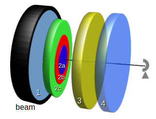
Fig. 3 Sketch of a distribution of core and foreground layers within the Gaussian shaped beam of the telescope (black ring). Here, we assume three different core components \(2a\), \(2b\), and \(2c\) located in a plane perpendicular to the line of sight which lies in front of the background layer \(1\) with intensity \(I_{\rm bg}^{\rm core}(\nu)\), see Eq. (8). The foreground layers \(3\) and \(4\) are located between the core layers and the telescope along the line of sight (black dashed line). Here, each component is described by different excitation temperatures, velocity offsets etc. indicated by different colors. The thickness of each layer is described indirectly by the total column density \(N_{\rm tot}^{m,c}\), see Sect. “Optical Depth”. For each foreground layer we assume a beam filling factor of 1, i.e. each foreground layer covers the whole beam.|
In contrast to core layers, foreground components may interact with each other, as shown in Fig. 3, where absorption takes places only, if the excitation temperature for the absorbing layer is lower than the temperature of the background.
Hence, the solution of the radiative transfer equation for foreground layers can not be given in a form similar to Eq. (12). Foreground components have to be considered in an iterative manner similar to Eq. (9). The solution of the radiative transfer equation for foreground layers can be expressed as
where \(m\) indicates the index of the current molecule and \(i\) represents an index running over all foreground components \(c\) of all molecules. Additionally, we assume that each foreground component covers the whole beam, i.e. \(\eta \left(\theta^{m,c=i} \right) \equiv 1\) for all foreground layer [11]. Thus, Eq. (13) simplifies to
where \(T_{\rm mb}^{\rm core}(\nu)\) describes the core spectrum, see Eq. (12), including the beam-averaged continuum background temperature \(I_{\rm bg}^{\rm core} (\nu)\). For foreground lines the contribution by other components is considered by first calculating the contribution of core objects and then use this as new continuum for foreground lines reflecting the fact that cold foreground layers are often found in front of hotter emission sources. The myXCLASS function assumes, that the cosmic background describes together with the core components one end of a stack of layers. Additionally, the foreground components are located between this plane and the telescope, see Fig. 3. The total column density \(N_{\rm tot}^{m,c}\) depends on the abundance of a certain molecule and on the thickness of a layer containing the molecule. The order of components along the line of sight is defined by the occurrence of a certain foreground component in the molfit file.
Stacking
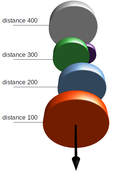
Fig. 4 Sketch of components located at different distances along the line of sight.
In addition to the simple 1-d description described in the previous
section, XCLASS offers the possibility to define the order of each
component along the line-of-sight by a so-called stacking or
distance parameter which replaces column CFFlag in the molfit
file, i.e. the column CFFlag is replaced by column distance
right after column V_off. The stacking parameter can be interpreted
as distance of a component to the observer where the component(s) with
the largest distance parameter is (are) closest to the background while
those components with the smallest distance parameter are closest to the
observer. Additionally, the components which have the same distance
parameter (i.e. within a difference of \(< 10^{-9}\)) are located in
the same plane perpendicular to line-of-sight. In contrast to foreground
components, described in the previous section, which can describe only
one molecule at a certain distance, the stacking formalism offers the
possibility to describe an arbitrary number of clouds consisting of an
arbitrary number of molecules, recombination lines, or continuum
contributions (like dust or synchrotron) along the line-of-sight.
SO2;v=0;   4

% s_size:  T_rot:   N_tot:   V_width:   V_off: distance:  keyword:
%[arcsec]     [K]   [cm-2]     [km/s]   [km/s]        []

   500.00   50.00  1.9E+14       2.86     1.22     600.0
   500.00  190.00  3.9E+15       4.16    -1.61     500.0
   500.00  250.00  3.9E+16       8.55    -5.75     500.0
   500.00   80.00  3.9E+14       1.23    -1.82     300.0

CH3CN;v=0;   2

% s_size:  T_rot:   N_tot:   V_width:   V_off: distance:  keyword:
%[arcsec]     [K]   [cm-2]     [km/s]   [km/s]        []

   500.00   50.00  2.2E+15       2.86     6.01     600.0
   500.00   80.00  8.5E+14       1.23    -2.82     200.0
Sub-beam description
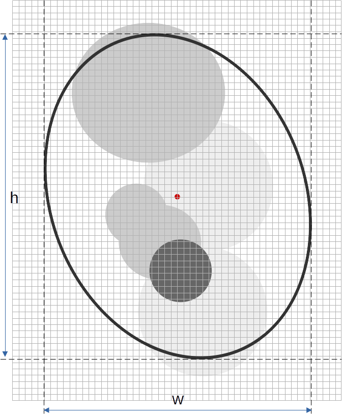
Fig. 5 Sketch of a sub-beam description for a single frequency channel. Here, the gray grid indicates the model grid, the black ellipse the beam, and the red dot the center of the beam, respectively. Additionally, the filled circles indicate different components, where the gray scale represent the location of a component along the line-of-sight, i.e. light gray describe components close the cosmic microwave background, while dark gray represents components close the observer. The projected width \(w\) and height \(h\) of the beam are described by Eq. (15).
Besides to the aforementioned component stacking XCLASS offers the possibility to take the shape and the position of each component perpendicular to the line-of-sight into account as well, see Fig. 4. The so-called sub-beam description, see Fig. 5, is used whenever an offset position of a component is defined, or if a component at a smaller distance is smaller than a component at larger distance, or if local-overlap is taken into account. Each component can have a different size and center position. In the current version only circle and square-shaped components can be described. Additionally, elliptical rotated beam sizes, see Sect. “Elliptical rotated Gaussians”, can be defined as well, but the frequency dependence of single dish beam sizes is ignored, i.e. the beam size is assumed to be constant for the whole frequency range [12]. For the sub-beam description, XCLASS samples the elliptical rotated beam by an rectangular linear grid, called model grid, where the number of pixels along the x- and y-direction is defined by the user. The size of each model pixel is defined by the beam, where we assume that the grid along the x- and y-axis is three times the width \(w\) and height \(h\) of the beam, respectively, described by
Here, \({\tt BMIN}\) and \({\tt BMAJ}\) represents the minor and major axis and \({\tt BPA}\) the position angle of the beam. Furthermore, XCLASS identifies for each component the model pixels, which are covered by the corresponding component. While the identification of all pixels covered by a component is trivial for square components, the Bresenham’s circle algorithm [Bresenham_1977] is used for circular components. After this, XCLASS computes the spectra for each model pixel based on the corresponding component configuration. Afterwards, XCLASS convolves the calculated intensity map for each frequency channel with the elliptical rotated Gaussian beam using the FFTW library [13] [Padua_2011]. Finally, XCLASS uses the spectrum at the beam center for the final output. The intensities and optical depths for each component / distance are computed in the same way.
For beam-centered components only the diameter of the component (in
arcsec) is required which has to be defined in the first column
s_size of the molfit file, e.g.
SO2;v=0;   4

% s_size:  T_rot:   N_tot:   V_width:   V_off: distance:  keyword:
%[arcsec]     [K]   [cm-2]     [km/s]   [km/s]        []

    50.00   50.00  1.9E+14       2.86     1.22     600.0
   110.00  190.00  3.9E+15       4.16    -1.61     500.0
s_off_x and
s_off_y describe the x- and y-coordination of the component center
position relative to the beam center (in arcsec), respectively.
Additionally, column (keyword) has to contain the keyword
circleoff.SO2;v=0; 2
% s_size: s_off_x: s_off_y: T_rot: N_tot: V_width: V_off: distance: keyword:
%[arcsec] [arcsec] [arcsec] [K] [cm-2] [km/s] [km/s] []
50.00 1.0 1.45 50.00 1.e14 2.86 1.22 600.0 circleoff
200.00 90.00 3.e15 4.16 -1.61 500.0
Additionally, the user can use keywords box and boxoff to define
quadratic components. For keyword box, XCLASS assumes that the
corresponding component is located at the center of the beam, where
column s_size indicates the length (in arcsec) of the square.
Similar to keyword circleoff the keyword boxoff defines a square
which center (in arcsec) is defined by columns s_off_x and
s_off_y, respectively.
Non-LTE description of molecules
In addition to the local thermodynamic equilibrium (LTE) description, XCLASS offers the possibility to treat molecules in Non-LTE as well using the RADEX routines [van_der_Tak_et_al_2007]. In the following we briefly describe the underlying formalism, using [van_der_Tak_et_al_2007] and the RADEX manual [14].
In general, collisions between atoms or molecules can cause transitions from any state \(i\) to any other state \(j\). In dense environments these collisions take place so often that the occupation numbers \(n_i\) and \(n_j\) are thermally distributed, i.e. they are described by the Boltzmann distribution where the Boltzmann temperature is identical to the kinetic temperature. If the density is very low, the radiative transitions can become more frequent than collisional transitions which requires a Non-LTE description.
In order to calculate the level populations we assume that for every level \(i\) the rate at which atoms/molecules are being (de-)excited out of level \(i\) is equal to the rate at which level \(i\) is being re-populated by (de-)excitation from other levels:
where \(P_{ji}\) describes the formation rate coefficient of level \(i\), while \(P_{ij}\) is the corresponding destruction rate coefficient which is given by
Thus we get
where \(A_{ij}\) indicates the probability for spontaneous emission, \(B_{ji} \, u_{ij}\) the probability for absorption, and \(B_{ij} \, u_{ij}\) the probability for induced emission. Additionally, the local radiative energy density \(u_{ij}\) is given by
where \(I_\nu\) represents the radiation field and \(\phi_{ij} \left(\nu\right)\) the line profile function for transition \(i \rightarrow j\). Furthermore, the \(C_{ij}\) describe the collision rates per second per molecule of the species of interest. They have to depend on the density of the collision partner, so that they can be expressed as \(C_{ij} = K_{ij} \, n_{\rm col}\), where \(n_{\rm col}\) indicates the density of the collision partner, which is in most cases H\(_2\). (XCLASS offers the possibility to define up to seven different collision partners for each distance, see Sect. “The collision partner file”.) The collisional rate coefficients \(K_{ij}\) (described in cm\(^3\) s\(^{-1}\)) are the velocity-integrated collision cross sections,
where \(E\) represents the collision energy, \(T_{\rm kin}\) the kinetic temperature, and \(\mu\) the reduced mass of the system. If collisions dominate \((n_j \, C_{ij} \gg A_{ij} + B_{ij} u_{ij})\), the upward rates are obtained through detailed balance
The \(K_{ij}\) depend on the temperature through the relative velocity of the colliding molecules and possibly also through the collision cross sections directly. The collision rates can be interpreted as the “collisional analogs” to the Einstein relations. [15]
For some cases, Eq. (16) can be expressed by the Boltzmann distribution of a specific temperature: If collisions dominate \((n_j \, C_{ij} \gg A_{ij} + B_{ij} u_{ij})\) the level populations are described by
where \(\Delta E_{ji} = E_j - E_i\) indicates the energy difference between both levels and \(T_{\rm kin}\) the kinetic temperature.
If radiation dominates \((n_j \, C_{ij} \ll A_{ij} + B_{ij} u_{ij})\) the level populations can be expressed as
where \(u_{ij} = B_\nu (T_{\rm rad})\) was assumed in the last step. For a given temperature, one can define the critical number density
as the density above which the collisions are so frequent, that LTE can be used, while below which there are substantial deviations from LTE.
But in many cases \((n_j \, C_{ij} \approx A_{ij} + B_{ij} u_{ij})\) and one defines an excitation temperature through
Assuming that \(u_{ij} = B_\nu (T_{\rm bg})\) , with \(T_{\rm bg}\) = 2.73 K representing the temperature of the cosmic microwave background, we can describe the excitation temperature \(T_{\rm ex}\) as
Note, that different lines will have different excitation temperatures.
But, in general, the radiation field is not described by the Planck function. Additionally, Eq. (16) is a local equation (to be solved at each location separately), but it has a global character due to the dependency on \(u_{ij}\) and \(u_{ji}\) which can be solved, usually with some simplifying assumptions.
The problem is how to “decouple” the radiative transfer calculations from the calculations of the level populations. A popular approach for this is the so-called escape probability method. The basic idea is to invent a factor that determines the chance that a photon at some position in the cloud can escape the system. This probability \(\beta\) depends only on the optical depth \(\tau\) and is related to the intensity within the medium, ignoring background radiation and any local continuum through
where \(S_{ij}\) describes the source function
The source function \(S_{ij}\) is independent of \(\nu\), at least over the small frequency range across the transition \(i \rightarrow j\) and has a single value for each line. (\(S_{ij} = B_{\nu_{ij}}(T)\) for LTE).
Note, that if all the photons escape, then \(\beta = 1\) and \(u_{ij}\) is the blackbody radiation field intensity. If no photons escape from the cloud, then \(u_{ij}\) is the source function.
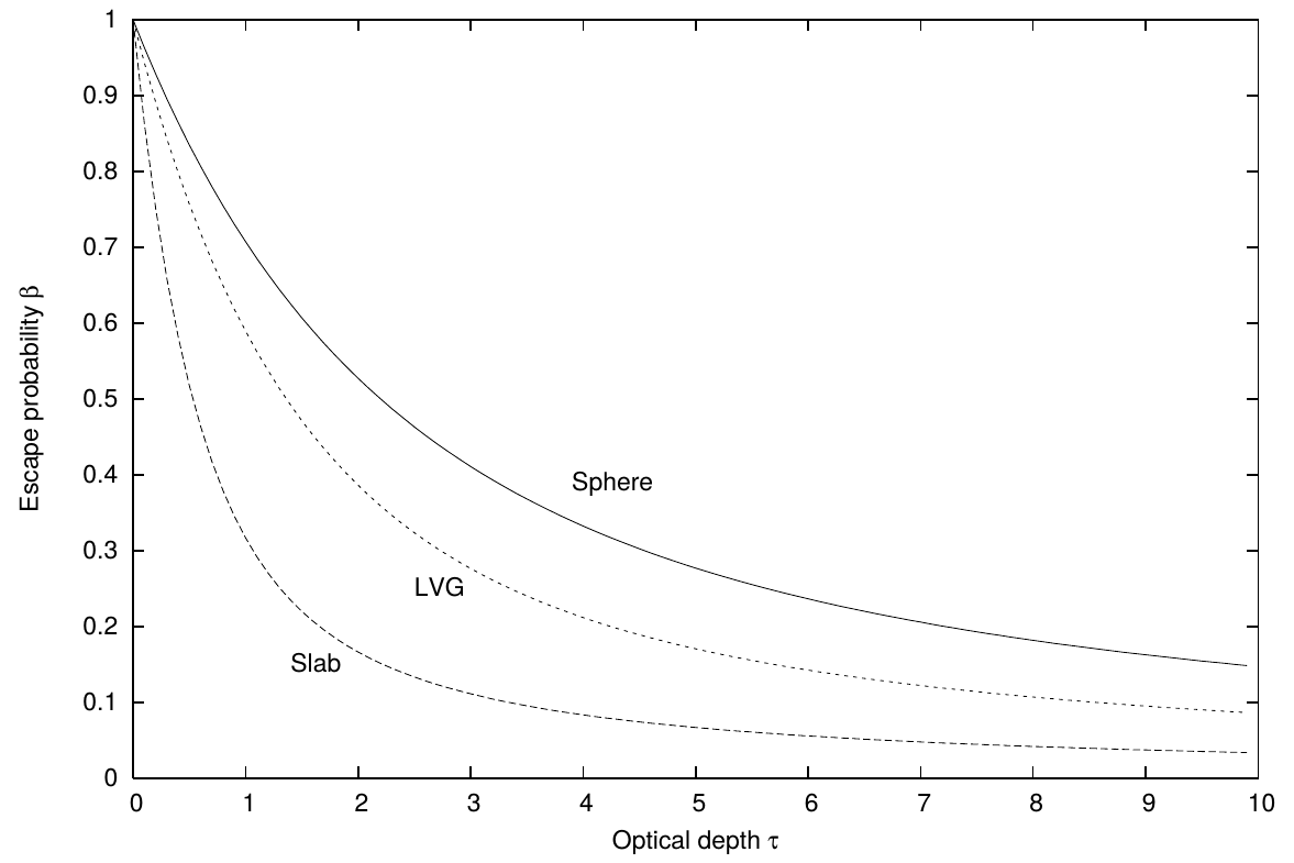
Fig. 6 Escape probability \(\beta\) as a function of optical depth \(\tau\) for three different geometries: uniform sphere (solid line), expanding sphere (dotted line) and plane-parallel slab (dashed line). (Taken from [van_der_Tak_et_al_2007]).
There are detailed relations between \(\beta\) and \(\tau\) for specific geometrical assumptions, see Fig. 6. The expression derived for an expanding spherical shell, the so-called Sobolev or large velocity gradient (LVG) approximation [Sobolev_1960] , [Castor_1970] , [Elitzur_1992]. This method is also widely applied for moderate velocity gradients, to mimic turbulent motions. RADEX uses the formula by [Mihalas_1978] and [Boland_De-Jong_1982] for this geometry:
For a homogeneous slab is found:
Also for a turbulent medium an escape probability has been estimated:
Finally for a uniform sphere
RADEX uses this last formula to estimate the excitation and radiation field in the following way. (For high optical depth, only the first term of the formula is retained; at low optical depth, a power series approximation is used.) As a first guess the level populations in the optically thin case (or for LTE) are calculated; this then gives the optical depth and hence the escape probability, from which the new level populations can be directly calculated. The program iterates this procedure to find a consistent level population and optical depth, and computes all line strengths for that solution.
The optical depth \(\tau_0\) in the line at line center is related to the populations by
where \(N_{\rm mol}\) is the total column density, \(\Delta V\) the full width at half-maximum of the line profile in velocity units, and \(x_l\) the fractional population of level \(l\). The formalism is analogous to the LVG method, with the global \(n/(dV/dR)\) replaced by the local \(N/\Delta V\).
The calculations proceed as follows. A first guess of the populations of the molecular energy levels is produced by solving statistical equilibrium in the optically thin case. The only radiation taken into account is the unshielded background radiation field; internally produced radiation is not yet available. The solution for the level populations allows calculation of the optical depths of all the lines, which are then used to re-calculate the molecular excitation. The new calculation treats the background radiation in the same manner as the internally produced radiation. The program iteratively finds a consistent solution for the level populations and the radiation field. When the optical depths of the lines with \(\tau > 10^{-2}\) are stable from one iteration to the next to a given tolerance (default 10\(^{-6}\)), the program writes output and stops.
RADEX includes some limitations. First of all only one molecule is treated at a time, so that the effects of line overlap are not taken into account. In special cases, overlap between lines of the same molecule may influence their excitation, for example the hyperfine components of HCN. By taking local-overlap into account, see Sect. “Local-overlap of neighboring lines”, XCLASS is able to overcome this limitation.
For certain molecules under certain physical conditions (especially low density and/or strong radiation field), population inversions occur, which cause negative optical depth and hence nonlinear amplification of the incoming radiation [Elitzur_1992]. This phenomenon, known as “maser” action, requires non-local treatment of the radiative transfer, in particular a fine sampling of directions. Generally, the escape probability approximation is justified until the masers saturate, which occurs at \(\tau \approx -1\). In practice, the computed intensities of lines with \(\tau \leq -0.1\) are not as accurate as those of other lines, and the intensities of lines with \(\tau \leq -1\) should be disregarded altogether. If many lines have negative optical depths, the intensities of non-maser lines may also be affected. RADEX may well be used to predict which lines of a molecule may display maser action under certain physical conditions. Note however that lines may be masers even if \(\tau > 0\) according to RADEX, for example “Class II” CH\(_3\)OH masers which are pumped by infrared radiation.
XCLASS uses the RADEX routines to compute the optical depths (multiplied with the user-defined line profile function) and the corresponding excitation temperatures for all transitions of a certain molecule and component, where the kinetic temperature, column density, line width and velocity offset of the corresponding component are used as input for RADEX. For components which are closest to the background, XCLASS uses the beam-averaged continuum background temperature \(I_{\rm bg} (\nu)\), Eq. (8), in conjunction with dust, free-free, and synchrotron continuum contributions as radiation field for RADEX. For components with smaller distance parameters, a radiation field caused by components at larger distances is used as input for the RADEX routines. So non-local effects are taken into account as well which partly removes the limitation of RADEX.
In order to describe a component of a certain molecule in Non-LTE the
keyword Non-LTE has to be added to column keyword for the
corresponding component. In the following example, we describe the first
component in Non-LTE:
CH3OH;v=0;   1
% s_size:  T_rot:   N_tot:  V_width:   V_off:  CFFlag:  keyword:
%[arcsec]     [K]   [cm-2]    [km/s]   [km/s]    [c/f]
    48.47   50.00  3.9E+16      2.86    -2.53        c   Non-LTE
But, the Non-LTE description requires the collision rates for the corresponding molecules and the density of the collision partners as well.
The collision partner file
These parameters are described by the so-called collision partner
file, where the first line indicates the used approximation for the
escape probability \(\beta\) (Geometry = 1 for an uniform sphere
described by
Eq. (20),
Geometry = 2 for an expanding spherical shell,
Eq. (18), and
Geometry = 3 for a homogeneous slab,
Eq. (19)). The
second line describes the number of molecules, which have at least one
component described in Non-LTE. The following lines describe for each
molecule the name of the molecule [16], and the path and name of the
so-called molecular data file, see below. Thereafter, two lines are
required for each collision partner: One line describes the name of the
collision partner (H2, p-H2, o-H2, e, H, He, and
H+), see below. The second line indicates the initial density (in
cm\(^{-3}\)), the lower and upper limit of the density (used for
fitting), and the corresponding distance in the molfit file,
respectively. If no distance is specified, the corresponding density is
used for all distances where the corresponding molecule is described in
Non-LTE. Additionally, two collision partners with a fixed ratio between
both densities can be defined as well, see below.
In the following example, we use the escape probability approximation
for an expanding spherical shell (Geometry = 2) and describe two
molecules CH\(_3\)OH-A and CO, with collision rates stored in
files "a-ch3oh.dat" and "co.dat", respectively. For
CH\(_3\)OH-A, we use two collision partners: H\(_2\)
(H2) and electrons (e). As mentioned above, XCLASS offers the
possibility to define the density of collision partners for different
distances and to fit these densities (here, between 1 cm\(^{-3}\)
and 10\(^5\) cm\(^{-3}\)) as well using the myXCLASSFit
function. Here, H\(_2\) has a initial density of
10\(^2\) cm\(^{-3}\) at distance 10\(^{10}\) and a
density of 10\(^4\) cm\(^{-3}\) at distance
10\(^{9}\). Additionally, we define a global density, i.e. a
density for all distances, of 5 cm\(^{-3}\) for electrons. For CO,
H\(^+\) is used as collision partner with an initial global
density of 10 cm\(^{-3}\) for all distances.
2                    % Geometry (=1: sphere, =2: LVG, =3: slab)
2                    % number of molecules in molfit file described in Non-LTE
CH3OH;v=0;A          % 1st molecule (with at least one component in Non-LTE)
a-ch3oh.dat          % path and name of file containing molecular data
3                    % number of collision partners for CH3OH;v=0;A
H2                   % first collision partner for CH3OH;v=0;A
1.e2 1.0 1.e5 1.e10  % density of 1st coll. partner (cm-3) at distance 1.e10
H2                   % second collision partner for CH3OH;v=0;A
1.e4 1.0 1.e5 1.e09  % density of 1st coll. partner (cm-3) at distance 1.e09
e                    % third collision partner for CH3OH;v=0;A
5.0  1.0 1.e5        % density of 2nd coll. partner (cm-3) (for all distances)
CO;v=0;              % 2nd molecule (with at least one component in Non-LTE)
co.dat               % path and name of file containing molecular data
1                    % number of collision partners for CO
H+                   % first collision partner (for CO)
1.e1 1.0 1.e5        % density of 1st coll. partner (cm-3) (for all distances)
H2), p-H\(_2\)
(p-H2), o-H\(_2\) (o-H2), electrons (e), H-atoms
(H), He (He), and H\(^+\) (H+). The user has to make
sure that the collisional data file contains collision rate
coefficients for all partners for which densities are given here. In
most cases, using H\(_2\) as only partner is a good default.
When H\(_2\) is given as collision partner for CO, a thermal
average of ortho and para H\(_2\) is taken.\[n_{\rm cp1} + n_{\rm cp2} = n_{\rm total}.\]The density \(n_{\rm cp1}\) of collision partner 1 is defined as
(21)\[n_{\rm cp1} = \frac{1}{1 + r} \cdot n_{\rm total},\]while the density \(n_{\rm cp2}\) of collision partner 2 is given as
(22)\[n_{\rm cp2} = \frac{r}{1 + r} \cdot n_{\rm total}.\]As in the non-fixed case, the density can be adjusted within the given range and/or also defined for a given distance.
2                    % Geometry (=1: sphere, =2: LVG, =3: slab)
1                    % number of molecules in molfit file described in Non-LTE
CH3OH;v=0;A          % 1st molecule (with at least one component in Non-LTE)
a-ch3oh.dat          % path and name of file containing molecular data
1                    % number of collision partners for CH3OH;v=0;A
p-H2 o-H2 3.0        % collision partners for CH3OH;v=0;A
1.e2 1.0 1.e5 1.e10  % density of 1st coll. partner (cm-3) at distance 1.e10
3.0 and a total density of
100 cm\(^{-3}\). Using Eqn. (21),
(22) the
densities of para- and ortho-H\(_2\) are 25 and
75 cm\(^{-3}\), respectively. Please note that here the line
with a fixed density ratio counts only as one, although two collision
partners are used.If you need to make your own molecular data file, here is a detailed description of the required file format. The format can be used for all molecules, whether linear (HCO\(^+\)) or not (H\(_2\)O). The lines that start with an exclamation mark (!) are not read by the program.
% Lines 1 - 2: molecule name
% Lines 3 - 4: molecular weight (a.m.u.)
% Lines 5 - 6: number of energy levels (NLEV)
% Lines 7 - (7 + NLEV): level number, level energy (cm-1), statistical
               weight. These numbers may be followed by additional
               info such as the quantum numbers, which are however
               not used by the program. The levels must be listed
               in order of increasing energy.
% Lines (8+NLEV) - (9+NLEV): number of radiative transitions (NLIN)
% Lines (10+NLEV - (10+NLEV+NLIN): transition number, upper level,
               lower level, spontaneous decay rate (s-1). These numbers may
               be followed by additional info such as the line frequency and
               upper state energy, which is however not used by the program.
% Lines (11+NLEV+NLIN) - (12+NLEV+NLIN): number of collision partners
% Lines (13+NLEV+NLIN) - (14+NLEV+NLIN): collision partner ID and reference.
               Valid identifications are: 1=H2, 2=para-H2, 3=ortho-H2,
               4=electrons, 5=H, 6=He, 7=H+.
% Lines (15+NLEV+NLIN) - (16+NLEV+NLIN): number of transitions for which
                                         collisional data exist (NCOL)
% Lines (17+NLEV+NLIN) - (18+NLEV+NLIN): number of temperatures for which
                                         collisional data exist
% Lines (19+NLEV+NLIN) - (20+NLEV+NLIN): values of temperatures for which
                                         collisional data exist
% Lines (21+NLEV+NLIN) - (21+NLEV+NLIN+NCOL): transition number, upper level,
               lower level; rate coefficients (cm3 s-1) at each temperature.
               RADEX interpolates between rate coefficients in the specified
               temperature range.
Outside this range, it assumes the collisional de-excitation rate coefficients are constant with T, i.e. it uses rate coefficients specified at the highest T (400 K in this case) also for higher temperatures, and similarly at temperatures below the lowest value (10 K in this case) for which rate coefficients were specified.
Radio recombination lines (RRLs)
In addition to molecules myXCLASS can deal with radio recombination lines (RRLs) as well. The description can be done in LTE as well as in Non-LTE.
RRLs in LTE
The optical depths of RRLs (in LTE) is given by [19]
where the LTE source function \(S_{{\rm RRL}, \nu}^{\rm LTE}\) can be written in terms of the brightness temperature Eq. (4) as
The terms \(n_1\), \(f_{n_1, n_2}\), \(E_{n_1}\), and \(\nu_{n_1, n_2}\) are taken from the embedded database whereas the emission measure EM (in cm\(^{-6}\) pc), electronic temperature \(T_e\) (in K), source size \(\theta^{m,c}\) (in arcsec) (or other parameters related to source description), line width \(\Delta v\) (in km/s), and velocity offset \(v\) (in km/s) used for the line profile function \(\phi_\nu\) are taken from the user-defined molfit file.
The parameters which are used for the description of radio recombination
lines (RRLs) are quite similar to the parameters used for molecules.
Here, the kinetic temperature is interpreted as electronic temperature
(in K) and the column density as emission measure EM (in
pc cm\(^{-6}\)). RRLs of hydrogen are marked as RRL-H, of
Helium as RRL-He, of Carbon as RRL-C, of Nitrogen as RRL-N,
and of Oxygen as RRL-O. In the following example we describe RRLs of
hydrogen at two distances with a Gaussian line shape:
RRL-H    2
% s_size:     T_e:   EM_RRL:  V_width:   V_off:  distance:
500.00000    6.9e4   5.5E+16       1.3      2.0      2.e15
500.00000    2.3e4   2.3E+12       2.5      2.0      1.e15
RRLs in Non-LTE

Fig. 7 Departure coefficients \(b_n\) derived by [Storey_Hummer_1995] for Hn\(\alpha\) lines for an electronic temperature of \(T_e\) = 10 000 K, and different densities.
In the previous case the Saha-Boltzmann distribution was used, see Sect. “Radio recombination lines, to determine the electron population. In the Non-LTE case, the radiative transitions are dominating over collisional transitions. In order to describe these departures one introduces for each electronic level \(n\) a so-called departure coefficient \(b_n\) relating the electron population in Non-LTE \(N_n\) with the LTE case \(N_n^*\),
These departure coefficients have been derived by [Storey_Hummer_1995], see Fig. 7, and depend on both collisional and radiative processes. XCLASS uses their tabulated coefficients [20] for optical thin and optical thick (default) HII-regions for all RRLs. Due to the fact that the departure coefficients depends on the electron density, the Non-LTE description of the RRLs requires an additional parameter, the electron density \(N_e\) (in cm\(^{-3}\)) for each component. Using the departure coefficients the Non-LTE source function \(S_{{\rm RRL}, \nu}^{\rm Non-LTE}\) can be expressed as
where
For \(b_{n_1} =b_{n_2} = 1\) Eq. (25) reduces to the LTE expression (24).
The hot plasma in HII regions gives rise to the emission of thermal
bremsstrahlung which causes a continuum opacity which will be described
in Sect. “Free-free contribution”. If the input parameter
t_back_flag indicates a phenomenological continuum description
(t_back_flag = True, \(\gamma \equiv 0\)) the free-free
contribution to the continuum is neglected. For a physical description,
i.e. (t_back_flag = False, \(\gamma \equiv 1\)) this
contribution is taken into account, see Sect.
“Free-free contribution”.
The description of radio recombination lines in Non-LTE in the molfit
ifle requires two additional parameters: the electron density (in
cm\(^{-3}\)), which is given in a column right after the emission
measure (N_e), and the keyword non-lte in an additional column
at the end of the line. In order to use departure coefficients
[Storey_Hummer_1995] for optical thin lines the column keyword
has to contain keyword thin as well. In the next example, we
describe the first component of the example mentioned above in Non-LTE,
while the second component is described still in LTE:
RRL-H    2
% s_size:   T_e:  EM_RRL:   N_e:   V_width:   V_off:  distance:   keyword:
500.00000  6.9e4  5.5E+16  5.1e9        1.3      2.0      2.e15    non-lte
500.00000  2.3e4  2.3E+12               2.5      2.0      1.e15
Line profile function
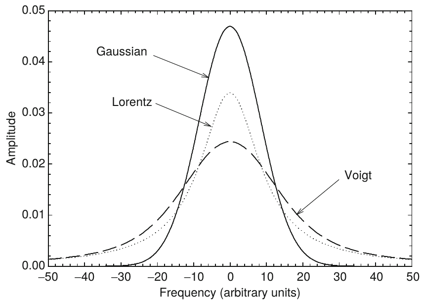
Fig. 8 Comparison of Gaussian, Lorentz, and their convolution (Voigt) line profiles. Each profile has the same area. The full widths at half-intensity are 20 for the Gaussian and Lorentz profiles, and 35 for the resulting Voigt profile. (Taken from [Lines_2002]).
XCLASS offers the possibility to use four different line profile functions to describe the line profile of each component which are briefly described in the following.
Lorentzian line profile
The normalized, i.e. \(\int_0^{\infty} \phi^{m,c,t}_{\rm Lorentz}(\nu) \, d\nu\) = 1, (Cauchy-) Lorentzian profile can be written as
where
describes the Doppler-shifted transition frequency \(\nu^t\) and \(\delta^{m,c,t} = f_L / 2\) the half-width at half-maximum which is related to the full width at half maximum \(f_L\) by
Additional, \(\Delta {\rm v}_{\rm width-Lorentz}^{m,c}\) and \(\delta {\rm v}_{\rm offset}^{m,c}\) indicates the line width and offset of molecule \(m\) and component \(c\), respectively and \({\rm v}_{\rm LSR}\) the source velocity.
In order to describe a component with a Lorentzian line shape the
keyword Lorentz has to be added to column keyword for the
corresponding component. The line width (defined in column V_width)
is now interpreted as Lorentz line width
\(\Delta {\rm v}_{\rm width-Lorentz}^{m,c}\). In the following
example, we describe the first component with a Lorentzian line shape,
while the second component uses a Gaussian line shape:
SO2;v=0;   2

% s_size:  T_rot:   N_tot:  V_width:   V_off:  CFFlag:  keyword:
%[arcsec]     [K]   [cm-2]    [km/s]   [km/s]    [c/f]
    48.47   50.00  3.9E+16      2.86    -2.53        c   Lorentz
    29.08   68.44  2.0E+17      4.02     0.22        f
Gaussian line profile
In order to take broadening caused by the thermal motion of the gas particles and micro-turbulence into account a normalized Gaussian line profile, i.e. \(\int_0^{\infty} \phi^{m,c,t}_{\rm Gauss}(\nu) \, d\nu\) = 1, for a spectral line \(t\) can be assumed:
where \(\nu_0^{m,c,t}\) indicates the Doppler-shifted transition frequency described by Eq. (27) and \(\sigma^{m,c,t}\) the standard deviation which is related to the full width at half maximum \(f_G\) by
Similar to the Lorentzian line profile \(\Delta {\rm v}_{\rm width-Gauss}^{m,c}\) and \(\delta {\rm v}_{\rm offset}^{m,c}\) indicates the line width and offset of molecule \(m\) and component \(c\), respectively and \({\rm v}_{\rm LSR}\) the source velocity.
The myXCLASS function assumes a Gaussian line shape for all
components by default. (In order to explicitly describe a component with
a Gaussian line shape, the keyword Gauss has to be added to column
keyword for the corresponding component.)
Voigt profile
The Voigt profile is a convolution of the Gaussian and the Lorentzian function, i.e.
The integral can not be solved analytically, but the Voigt function can be identified as real part of the Feddeeva function
with argument
i.e.
Due to the fact that the computation of the Voigt profile is computational quite expensive, XCLASS uses the pseudo-Voigt profile which is an approximation of the Voigt profile \(V(x)\) using a linear combination of a Gaussian \(G(x)\) and a Lorentzian line profile function \(L(x)\) instead of their convolution.
The mathematical definition of the normalized, i.e. \(\int_0^{\infty} \phi^{m,c,t}_{\rm pseudo-Voigt}(\nu) \, d\nu\) = 1, pseudo-Voigt profile is given by
where \(f_L\) and \(f_G\) represents the Lorentzian Eq. (28) and Gaussian Eq. (29) full width at half maximum (FWHM), respectively. There are several possible choices for the \(\eta\) parameter. XCLASS use the simple formula [Thompson_et_al_1987]
where
which is accurate to 1%.
In the molfit file, the Voigt line profile requires three additional
columns (V_width_G, V_width_L, and keyword indicating the
Gaussian line width (in km s\(^{-1}\)), the Lorentz line width
(in km s\(^{-1}\)) and keyword Voigt, respectively) for each
component which is described with a Voigt line profile, while column
V_width is not needed. In the following example, the first
component of SO\(_2\) is described with a Voigt line profile,
while the second and third component use a Lorentzian and a Gaussian
line shape, respectively.
SO2;v=0;   3

% s_size: T_rot: N_tot: V_width: V_width_G: V_width_L:   V_off: CFFlag: keyword:
%[arcsec]    [K] [cm-2]   [km/s]     [km/s]     [km/s]   [km/s]   [c/f]
      50.00  50.00 3.E+16                2.86       1.12    -2.53       c Voigt
      50.00  99.24 6.E+17     1.02                           3.22       f Lorentz
      50.00  68.44 2.E+17     4.02                           0.22       f
For RRLs, there is a contribution due to the broadening of the electronic levels in regions with high electron density. This is known as pressure broadening and it produces a Lorentzian profile. This broadening can be specified by the half-width at half-maximum height, \(f_L\), which has been computed numerically using analytic expressions that approximate the results derived from classical and semi-classical theory [Gee_et_al_1976] for the different quantum number ranges of the RRLs
Range of electronic levels |
Pressure broadening, \(f_L\) |
|---|---|
n \(>\) 100 |
1.9 \(\times\) 10\(^{-8} \, n^{4.4} \, N_ e / \left(Z^2 \, T_e^{0.1}\right)^a\) |
30 \(<\) n \(<\) 100 |
6.7 \(\times\) 10\(^{-9} \, n^{4.6} \, N_ e / \left(Z^2 \, T_e^{0.1}\right)^b\) |
n \(<\) 30 |
8.0 \(\times\) 10\(^{-10} \, n^{5} \, N_ e / \left(Z^2 \, T_e^{0.1}\right)^c\) |
In order to use the expressions described in Tab. “Analytic approximations of the pressure broadening for different ranges of electronic levels. References: (a) [Brocklehurst_Seaton_1972], (b) [Walmsley_1990] (c) [Strelnitski_et_al_1996].” for the pressure broadening for a specific component of a RRL, the Lorentzian line width has to be set to a negative value, e.g.
RRL-H   1

% s_size: T_rot: N_tot: V_width: V_width_G: V_width_L:   V_off: CFFlag: keyword:
%[arcsec]    [K] [cm-2]   [km/s]     [km/s]     [km/s]   [km/s]   [c/f]
    50.00  50.00 3.E+16                2.86       -1.0    -2.53       c Voigt
Horn profile

Fig. 9 Synthetic Horn line-profiles, for three different Horn H parameters. The full width at zero level is \(\Delta \nu\) = 8 km/s in all cases.
Horn line profiles [21] [Potter_et_al_2004] are like those encountered in envelopes of stars. They are parameterized by the transition frequency \(\nu_0^{m,c,t}\), the line width and the Horn to Center ratio. The aspect of the profile varies from parabola (as obtain in optically thick lines) for Horn/Center = -1 to flat-topped lines (unresolved optically thin lines) for Horn/Center = 0 and double peaked profiles (resolved optically thin lines) for Horn/Center > 0. Note, a Horn/Center parameter \(H < (-1)\) is not allowed. The profile is symmetric, normalized, i.e. \(\int_0^{\infty} \phi^{m,c,t}_{\rm Horn}(\nu) \, d\nu\) = 1, and is described by
where \(H\) represents the dimensionless Horn/Center parameter and \(f_H\) the full width at half maximum
where \(\nu_0^{m,c,t}\) again represents the Doppler-shifted transition frequency described by Eq. (27).
The Horn line profile requires three additional columns
(V_width_Horn_W, V_width_Horn_H, and keyword indicating the
Horn line width \(\Delta {\rm v}_{\rm width-Horn}^{m,c}\) (in km
s\(^{-1}\)), the Horn H parameter (dimensionless) and keyword
Horn, respectively) for each component which is described with a
Horn line profile, while column V_width is not needed. In the
following example, the first component of SO\(_2\) is described
with a Horn line profile.
SO2;v=0;   1

% s_size: T_rot: N_tot: V_width_Horn_W: V_width_Horn_H: V_off: CFFlag: keyword:
%[arcsec]    [K] [cm-2]          [km/s]              [] [km/s]   [c/f]
    50.00  50.00 3.E+16            2.86            1.12  -2.53       c Horn
Contributions to continuum

Fig. 10 Sketch of different continuum contributions of Arp 220-West. (Taken from [Downes_Eckart_2007]).
XCLASS offers the possibility to describe the dust, free-free, and synchrotron contribution to the continuum, see Fig. 10, self-consistently, where the different contributions are modeled by a set of parameters. These parameters can be defined globally for each frequency range or in the molfit file for each distance. For globally defined parameters, the myXCLASS function applies the continuum parameters only to the component with the largest beam filling factor, see Eq. (2), for each distance to avoid an overestimation.
Dust contribution
The dust optical depth \(\tau_d^{m,c}(\nu)\) takes the dust attenuation into account and is given by
Here, \(N_H^{m,c}\) describes the hydrogen column density (in
cm\(^{-2}\)), \(\kappa^{m,c}_{\nu_{\rm ref}}\) the dust mass
opacity for a certain type of dust (in cm\(^{2}\)
g\(^{-1}\)) [Ossenkopf_Henning_1994], and \(\beta^{m,c}\) the
spectral index. Additionally, \(\nu_{\rm ref}\) = 230 GHz indicates
the reference frequency for \(\kappa^{m,c}_{\nu_{\rm ref}}\),
\(m_{H_2}\) the mass of a hydrogen molecule, and
\(1 / \zeta_{\rm gas-dust}\) the dust to gas ratio which is set here
to (1/100) [Hildebrand_1983]. The equation is valid for dust and
gas well mixed. Furthermore, the expression
\(\tau_d^{\rm file}(\nu)\) represents the dust optical depth
described in an ASCII file, which path and name is defined by the input
parameter DustFileName.
On the one hand the dust parameters \(N_H^{m,c}\),
\(\kappa^{m,c}_{\nu_{\rm ref}}\), and \(\beta^{m,c}\) can be
defined globally for all components in the molfit file by the input
parameters N_H, kappa_1300, and beta_dust of the
myXCLASS function, while the dust temperature is set to the
excitation temperature of the corresponding component. For the
myXCLASSFit, myXCLASSMapFit, myXCLASSMapRedoFit, LineID,
and CubeFit function the dust parameters can be defined globally in
an obs. xml file as well, see Sect. “Observational xml file”.
Additionally, the dust parameters can be described in the molfit file
for different distances, while the dust continuum has to be marked as
cont-dust. Each component is described by the size of the dust
component s_size (in arcsec), the dust temperature T_cont_dust
(in K), the hydrogen column density nHcolumn_cont_dust (in
cm\(^{-2}\)), the dust mass opacity kappa_cont_dust (in g
cm\(^{-2}\)), the spectral index beta_cont_dust, and the
distance parameter distance. In the example described below, we
define four different dust components with different dust temperatures
at different distances
cont-dust    4
% s_size: T_cont_dust: nHcolumn_cont_dust: kappa_cont_dust: beta_cont_dust: distance:
500.00000       50.000             3.9E+16             0.42             2.0    4.e15
500.00000       10.000             1.2E+20             0.42             2.0    3.e15
500.00000       32.000             5.3E+12             0.42             2.0    2.e15
500.00000        5.000             7.1E+18             0.42             2.0    1.e15
In order to be backward compatible with older XCLASS releases, the user can define the dust parameters for each component of a molecule as well. Here, the dust temperature \(T_d^{m,c}\) is parameterized as offset to the corresponding excitation temperature \(T_{\rm ex}^{m,c}\) as
where \(T_{d, {\rm off}}^{m,c}\) and
\(T_{d, {\rm slope}}^{m,c}\) can be defined by the user for each
component in the molfit. If \(T_{d, {\rm off}}^{m,c}\) and
\(T_{d, {\rm slope}}^{m,c}\) are not defined for a certain
component, we assume
\(T_d^{m,c} (\nu) \equiv T_{\rm ex}^{m,c} (\nu)\) for all
components. For a physical (\(\gamma \equiv 1\)) description of the
background intensity, see
Eq. (5), the user
can define the dust opacity,
Eq. (32), and dust
temperature,
Eq. (33),
for each component. In order to define a dust temperature for each
component which is not identical to the excitation temperature
\(T_{\rm ex}\) of the corresponding component, the molfit file has
to contain two additional columns between columns V_off and
CFFlag (or column distance), describing the parameters
\(T_{\rm d, off}^{m,c}\) (T_doff) and
\(T_{\rm d, slope}^{m,c}\) (T_dSlope), respectively, and keyword
t-dust-inline in column (keyword), e.g.
CS;v=0;    3
% s_size: T_rot: N_tot: V_width: V_off: T_doff: T_dSlope: CFFlag: keyword:
%[arcsec]    [K] [cm-2]   [km/s] [km/s]     [K]        []   [c/f]
    48.47  50.00   3e16     2.86  -2.56     3.0       0.0       c t-dust-inline
    40.10  56.53   2e18     4.21  -7.31     3.0       0.0       c t-dust-inline
    29.09  68.44   2e17     4.02   0.21     2.5       1.0       c t-dust-inline
Additionally, the myXCLASS program offers the possibility to define
\(N_H\), \(\kappa_{\nu_{\rm ref}}\) and \(\beta\) for each
component of a molecule as well. In order to define these parameters
individually for each component, the molfit file has to contain three
additional columns on the left side of column CFFlag (or column
distance), indicating parameters \(N_H^{m,c}\) (nHcolumn),
\(\kappa^{m,c}_{\nu_{\rm ref}}\) (kappa), and
\(\beta^{m,c}\) (beta), and keyword nh-dust-inline in column
(keyword), e.g.
CS;v=0;    3
% s_size: T_rot: N_tot: V_width: V_off: nHcolumn:  kappa: beta: CFFlag: keyword:
%[arcsec]    [K] [cm-2]   [km/s] [km/s]    [cm-2] [cm2/g]    []   [c/f]
    48.47  50.00   3e16     2.86  -2.56      3e24    0.42   2.0       c nh-dust-inline
    56.53  20.00   2e18     4.21  -7.31      2e24    0.42   2.1       c nh-dust-inline
    68.44  90.00   2e17     4.02   0.21      3e21    0.42   1.9       c nh-dust-inline
T_doff),
\(T_{d, {\rm slope}}^{m,c}\) (T_dslope) have to be given
before the hydrogen column density, kappa and beta, i.e. in the order
of s_size, T_rot, N_tot, V_width, V_off,
T_doff, T_dslope, nHcolumn, kappa, beta, and
CFFlag. Additionally, the column (keyword) has to contain the
keyword t-dust-inline_nh-dust-inline.Free-free contribution
The optical depth of the free-free contribution in terms of the classical electron radius \(r_e = (\alpha \, \hbar \, c) / (m_e \, c^2) = \alpha^2 \, a_0\) is given by [22]
where the electron temperature \(T_e\) and the emission measure EM has to be defined by the user. Additionally, XCLASS uses the tabulated thermal averaged free-free Gaunt coefficients [23] \(\langle g_{\rm ff} \rangle\) derived by [Van_Hoof_et_al_2015], which include relativistic effects as well, see Fig. 11.

Fig. 11 Relativistic thermally averaged free-free Gaunt factors \(\langle g_{\rm ff} \rangle\) for different temperatures \(T_e\) as function of \(u = \hbar \, \omega / k_B \, T_e\), derived by [Van_Hoof_et_al_2015].
In the molfit file contributions of free-free transitions to the
continuum are indicated by the phrase cont-free-free. Each free-free
component is described by the size of the component s_size (in
arcsec) the electronic temperature Te_ff (in K) the emission measure
EM_ff (in pc cm\(^{-6}\)) and the distance. In the following
example, we describe the free-free contribution at three different
distances:
cont-free-free    3
% s_size:    Te_ff:     EM_ff:   distance:
500.00000     9.0e4     6.3E+5       9.e15
500.00000     4.2e4     3.9E+7       4.e15
500.00000     1.0e4     2.9E+3       1.e15
Similar to the dust contribution, the free-free continuum parameters
can be defined globally, by using the input parameters Te_ff and
EM_ff. For the myXCLASSFit, myXCLASSMapFit,
myXCLASSMapRedoFit, LineID, and CubeFit function the
free-free parameters can be defined globally in an obs. xml file as
well, see Sect. “Observational xml file”.
Bound-free contribution
In one of the next releases XCLASS will be able to describe the bound-free contribution to the continuum as well. Free-bound transitions contribute significantly to the NIR-emission of HII-regions. At NIR-frequencies the free-bound radiation dominates over free-free emission. Assuming LTE conditions, we can use Saha’s equation and obtain the Milne relation
[Karzas_Latter_1961] obtained for hydrogenic atoms the cross section
with a Gaunt factor \(g\left(\omega, n, l, Z\right)\) depending on the radial and angular quantum numbers \((n, l)\). This Gaunt factor is close to 1.
Integrating the number of emitted photons \(N_+ \, N_e \, \sigma_{\rm fb} \, f(v) \, v \, dv\) times \(h \, \nu \, \delta(\nu - \xi/h - m v^2 / 2)\) over the electron velocity distribution gives
which is the emissivity for radiative recombinations to states of radial quantum number \(n\). The spectral emissivity for all recombinations is the sum over all transitions to ionization energies \(\chi/n^2\) less than the photon energy. So
is the free-bound emissivity for hydrogenic ions of charge \(Z\). The sum included in Eq. (35) can be evaluated using the approximation of [Brussaard_Van_de_Hulst_1962].
In the molfit file contributions of bound-free transitions to the continuum are described by the free-free parameter, see Sect. “Free-free contribution” and can be computed only in conjunction with the free-free contribution.
Synchrotron contribution
Synchrotron radiation (also known as magnetobremsstrahlung radiation) is the electromagnetic radiation emitted when charged particles are accelerated radially, i.e., when they are subject to an acceleration perpendicular to their velocity. If the particle is non-relativistic, then the emission is called cyclotron emission otherwise the emission is called synchrotron emission. In astronomy, synchrotron radiation is produced by fast electrons moving through magnetic fields and has a characteristic polarization.
The emissivity \(\epsilon_{\rm sync}^{m,c}(\nu)\), see Eq. (5), of a power-law electron energy distribution \(N(E) = \kappa E^{-p}\) (expressed in electron m\(^{-3}\) GeV\(^{-1}\)) in the case of a random magnetic field is [24]
where
with
The absorption coefficient \(\kappa_{\rm sync}^{m,c} (\nu)\), see Eq. (5), for a random magnetic field is
where
The description of synchrotron radiation (see
Sect. “Synchrotron contribution”) in the molfit file is
indicated by cont-sync. Here, each component defines the size of the
component s_size (in arcsec) the energy of the electrons
kappa_sync (in electron m\(^{-3}\) GeV\(^{-1}\)), the
strength of the magnetic field B_sync (in Gauss), the spectral
energy index p_sync (dimensionless), the thickness of the slab
l_sync (in AU), and the distances distance. In the following
example, we model the synchrotron contribution at two different
distances:
cont-sync    2
% s_size:   kappa_sync:   B_sync:   p_sync:   l_sync:   distance:
500.00000         9.0e4    6.3E-7       3.3     1.e12        2.e9
500.00000         5.0e4    6.3E-7       3.3     1.e12        1.e9
Similar to the dust contribution, the synchrotron continuum parameters
can be defined globally, by using the input parameters kappa_sync,
B_sync, p_sync, and l_sync. For the myXCLASSFit,
myXCLASSMapFit, myXCLASSMapRedoFit, LineID, and the
CubeFit function the synchrotron parameters can be defined globally
in a obs. xml file as well, see Sect. “Observational xml file”.
Phenomenological continuum description
In addition to the the different continuum contributions described above, XCLASS offers the possibility to describe the continuum of a given distance by phenomenological functions. Currently, the following functions are included:
Standing wave (
ContPhenFuncID = 1):\[c(\nu) = A_1 \, \sin \left( (\nu \cdot x) + \phi_1 \right) + A_2 \, \cos \left( (\nu \cdot x) + \phi_2 \right),\]where \(A_{1, 2}\) and \(x\) describe scale parameters whereas \(\phi_{1,2}\) indicate phase shifts. Here, \(A_1\) and \(A_2\) are defined by parameters
ContPhenFuncParam1andContPhenFuncParam2, respectively. ParameterContPhenFuncParam3indicates the scale parameter \(x\) and the phase shifts \(\phi_{1,2}\) are described by parametersContPhenFuncParam4andContPhenFuncParam5, respectively.Planck function (
ContPhenFuncID = 2):\[c(\nu) = \frac{h \, \nu}{k_B}\frac{1}{e^{h \, \nu / k \, T} - 1},\]with temperature \(T\) described by input parameter
ContPhenFuncParam1. The other input parametersContPhenFuncParam2-ContPhenFuncParam5have to be set to zero.beam-averaged continuum background temperature (
ContPhenFuncID = 3):(38)\[c(\nu) = T_{\rm bg} \cdot \left(\frac{\nu}{\nu_{\rm ref}} \right)^{T_{\rm slope}},\]where \(\nu_{\rm ref}\) (described by input parameter
ContPhenFuncParam1) indicates the reference frequency (in MHz) for \(T_{\rm bg}\) (defined by input parameterContPhenFuncParam2). The temperature slope (unitless) \(T_{\rm slope}\) is defined by input parameterContPhenFuncParam3. If input parameterContPhenFuncParam4is set to zero Eq. (38) is applied to all frequency ranges. But the user can restrict the application of Eq. (38) to a given frequency range by using input parametersContPhenFuncParam1andContPhenFuncParam4, whereContPhenFuncParam1defines the first andContPhenFuncParam4the last frequency, respectively. The other input parameterContPhenFuncParam5must always be set to zero.Anomalous Microwave Emission (AME) (
ContPhenFuncID = 4):\[c(\nu) = {A_{\rm AME}} \cdot \mathrm{exp} \left[-\frac{1}{2} \cdot \left[ \frac{ \ln \left(\frac{\nu }{{\nu_{\rm AME}}} \right)}{W_{\rm AME}}\right]^2 \right],\]where \(A_{\rm AME}\) (described by input parameter
ContPhenFuncParam2) indicates the the maximum flux intensity (in K) due to AME, \(\nu_{\rm AME}\) (described by input parameterContPhenFuncParam3) the correspondent frequency (in MHz) for that maximum, and \(W_{\rm AME}\) (described by input parameterContPhenFuncParam4) the width (unitless) of the distribution on the log-log plane. For more details see e.g. [Stevenson_2014] and [Poojon_2024].CMB Emission (
ContPhenFuncID = 5):\[c(\nu) = \frac{x^2 \, \mathrm{e^x}}{(\mathrm{e}^x - 1)^2} \cdot \Delta {T_{\rm CMB}},\]where \(x = \left( h \, \nu / k_B \, T_{\rm CMB} \right)\) and \(\Delta T_{\rm CMB}\) (described by input parameter
ContPhenFuncParam2) models the CMB anisotropies (in K). Here \(T_{\rm CMB}\) is fixed to 2.72548 K. For more details see e.g. [Poojon_2024].
Note, the aforementioned continuum function \(c(\nu)\) is added to the background intensity of the corresponding distance.
In order to use a phenomenological description of the continuum in the
molfit file, the phrase cont-phen has to be used. Each component is
described by the source size s_size (in arcsec) (or
other parameters related to source description), the function-id
func-id, the input parameters p_1, p_2, p_3, p_4,
and p_5, representing the input parameters ContPhenFuncParam1 -
ContPhenFuncParam5 and the distance distance. In the example
describe below, we use an expression for a standing wave to describe the
continuum phenomenologically at a given distance:
cont-phen    1
% s_size:   func-id:   p_1:   p_2:   p_3:   p_4:   p_5:   distance:
500.00000          1    0.2    0.2    0.2    0.2    0.2       1.e20
Similar to the dust contribution, the phenomenological continuum
parameters can be defined globally, by using the input parameters
ContPhenFuncID, ContPhenFuncParam1, ContPhenFuncParam2,
ContPhenFuncParam3, ContPhenFuncParam4, and
ContPhenFuncParam5. For the myXCLASSFit, myXCLASSMapFit,
myXCLASSMapRedoFit, LineID, and CubeFit function the
phenomenological parameters can be defined globally in a obs. xml file
as well, see Sect. “Observational xml file”.
Derivations
Detection Equation
In absence of scattering, the radiative transfer equation
\[\frac{\mathrm{d} I_{\nu}}{\mathrm{d} s} = -\kappa_{\nu}(s) I_{\nu} + \epsilon_{\nu}(s)\]
describes the propagation of radiation which passes through a medium. During the propagation photons are absorbed and emitted indicated by the emission and absorption coefficients \(\epsilon_\nu\) and \(\kappa_{\nu}\), respectively.
The optical depth \(\tau_{\nu}(s)\) which measures the distance in units of the mean free path, is given by
By using the source function \(S_{\nu} = \frac{\epsilon_{\nu}}{\kappa_{\nu}}\), the radiative transfer equation can be expressed as
Within the local thermodynamic equilibrium (LTE) the source function is described by Planck’s law for black body radiation \(B_{\nu}(T)\). Integrating Eq. (40) over \(\tau\) leads to
\[I_{\nu}(s) = I_{\nu}(0) \, e^{-\tau_{\nu}} + \int_{\tau'=0}^{\tau'=\tau} S_{\nu}(\tau'_{\nu}) e^{\tau'_{\nu} - \tau_{\nu}} d \tau'_{\nu}.\]
Assuming a constant source function, i.e. constant emission and absorption coefficients through the medium, the transfer equation can be written as
Additionally, we have to take into account, that the different components may not cover the whole beam, i.e. that the background behind a certain component might contribute as well. So, we have to extend Eq. (41) by introducing the beam filling factor \(\eta\), Eq. (2), which describes the fraction of the beam covert by a component
Here, the term \(\eta \, I_{\nu}(0) \, e^{-\tau_{\nu}}\) indicates the attenuated radiation from the background \(I_{\nu}(0)\). The second term \(\eta \, S_{\nu} \left(1 - e^{-\tau_{\nu}} \right)\) describes the self attenuated radiation emitted by a certain component. Finally, the last term \(\left(1 - \eta\right) \, I_{\nu}(0)\) represents the contribution of the background which is not covert by a component.
In real observations, we do not measure absolute intensities but only differences of intensities, i.e. we have to subtract the OFF-position from Eq. (42) as well, where we have an intensity caused by the cosmic background \(J_\mathrm{CMB}\). So, we achieve
Beam Filling Factor

Fig. 12 a)~A single two-dimensional Gaussian function, Eq. (44), with \(\sigma_x = \sigma_y = 1.9\) and \(\mu_x = \mu_y = 0\) representing a Gaussian beam of a telescope. b)~Cut through the Gaussian function described in a) at half height. c)~A single two-dimensional Gaussian function, with \(\sigma_x = \sigma_y = 1.1\) and \(\mu_x = 0.5\) and \(\mu_y = 0.9\) representing a Gaussian beam of a point source. d)~Cut through the Gaussian function described in a) at half height. e)~Convolved Gaussian of telescope and point`source as given by Eq. (46). f)~Cut through the convolved Gaussian function described in e) at half height.
The derivation of the beam filling factor (2) starts with the normalized two-dimensional Gaussian function
where \(\sigma_x^2\) and \(\sigma_y^2\) describe the variances and \(\mu_x\) and \(\mu_y\) the center along the \(x\) and \(y\) axis, respectively.
Observing a Gaussian shaped extended source with a telescope is described by a convolution of two two-dimensional Gaussian functions:
Assuming that \(g_1\) describes the telescope with \(\mu_{x,1} = \mu_{y, 1} \equiv 0\) and that telescope and extended source are described by non-elliptical Gaussians, i.e. \(\sigma_{x,1} = \sigma_{y,1} \equiv \sigma_1\) and \(\sigma_{x,2} = \sigma_{y,2} \equiv \sigma_2\), Eq. (45) can be simplified to [25]
The FWHM of the resulting Gaussian is given by
which describe an area of
In the last line we used the relation between the variances \(\sigma_{1,2}\) and the user defined FWHM of telescope (\(\theta_1 \equiv \theta_t\)) and source size (\(\theta_2 \equiv \theta^{m,c}\)) which is given by
The beam filling factor Eq. (2) is defined as ratios of areas
which is completely independent of the position \(\mu_x\) and \(\mu_y\) of the extended source within the telescope beam.
If more extended sources are observed with the telescope, we have to convolve the already convolved Gaussian Eq. (46) with a further two-dimensional Gaussian function with variance \(\sigma_{x,3} = \sigma_{y,3} \equiv \sigma_3\) and center \(\mu_{x,3}\) and \(\mu_{y,3}\). We get
The FWHM of the resulting Gaussian is given by
which describe an area of
In the last line we used again the relation between the variances and FWHM, Eq. (49). Now, we can again define a beam filling factor similar to Eq. (2) and get
When we observe more than three extended sources with a telescope we have to iteratively convolve the resulting Gaussian with a further two-dimensional Gaussian function and we can generalize Eq. (53) to
where \(\theta_1 \equiv \theta_t\) describes the FWHM of the Gaussian shaped beam of the telescope, defined by the diffraction limit, Eq. (3).
Optical Depth

Fig. 13 Transitions between the lower \(l\) and the upper \(u\) level with the corresponding Einstein coefficients.
In order to derive Eq. (7) we consider a system which involves radiative transitions between a lower \(l\) and an upper \(u\) level only. As shown in Fig. 13 , the lower level has an energy \(E_l\) and the upper level an energy \(E_u > E_l\). With
describing the energy difference between these two levels we can express the emissivity due to spontaneous radiative decay as
where \(A_{u,l}\) describes the Einstein A-coefficient, or radiative decay rate for the transition from the lower \(l\) to the upper \(u\) level. The expression \(1 / A_{u,l}\) gives the averaged time, that a quantum mechanical system can stay in level \(u\) before radiatively decaying to level \(l\), where we assume no collisional (de-)excitation. The expression \(\phi_{l,u} (\nu)\) describes the line profile of the transition of photons of frequency \(\nu\) and is normalized to 1, i.e. \(\int_0^\infty \phi(\nu) \, d \nu = 1\).
Similar to Eq. (56) we can write the extinction coefficient, which describes the radiative excitation from the lower to the upper level
where \(B_{l,u}\) describes the Einstein B-coefficient for extinction.
In addition to spontaneous emission and extinction we have to take the stimulated emission into account, which can be described by adding a negative opacity contribution to Eq. (57):
where \(B_{u,l}\) represents the Einstein B-coefficient for stimulated emission. So, for \(n_l B_{l,u} < n_u \, B_{u,l}\) we get laser (maser) emission.
The different Einstein coefficients are related to each other by the Einstein relations:
Following Eq. (39), the differential optical depth \(\tau_{\nu}\) is defined as
where we used the Einstein relations Eqn. (59) in the last line. By assuming LTE conditions and therefore Boltzmann population distribution
we can rewrite Eq. (60) by using Eq. (55)
Finally, we have to integrate along the line of sight and obtain the optical depth \(\tau_{\nu}\)
where \(N_u = \int n_u \, ds\) describes the column density of a certain molecule in the upper state.
In order to express Eq. (62) in terms of the total column density \(N_{\rm tot} = \sum_{i=0}^\infty n_i\) we start again with the Boltzmann population distribution
where we used the partition function \(Q(T_{\rm ex})\), which is defined as sum over all states
For our purpose we rewrite Eq. (63) in terms of \(N_u\) and \(N_l\):
Inserting this expression into Eq. (62) gives
where we used Eq. (55) to achieve Eq. (7) for a single line of a certain component and molecule.
Radio recombination lines
In order to get the linear absorption coefficient we consider a system involving radiative transitions between to levels indicated by the quantum numbers \(n_1\) and \(n_2\), respectively. The corresponding level energies \(E_{n_1}\) and \(E_{n_2}\) are related by the transition frequency \(\nu_{n_1, n_2}\) with
where we assumed that \(E_{n_1} < E_{n_2}\). Now, we can write the extinction coefficient, which describes the radiative excitation from the lower (\(n_1\)) to the upper (\(n_2\)) level
where \(B_{n_1, n_2}\) represents the Einstein B coefficient for extinction and \(\phi_{n_1, n_2} (\nu)\) describes the normalized line profile (in units of Hz\(^{-1}\)) of the transition of photons of frequency \(\nu_{n_1, n_2}\).
In addition we take the stimulated emission into account, which can be described by adding a negative opacity contribution to (67):
where \(B_{n_2, n_1}\) indicates the Einstein B coefficient for stimulated emission.
Now we use the Boltzmann equation
and the well-known Einstein relation
to get
where the term in squared brackets describes the correction of the stimulated emission in thermodynamic equilibrium.
Now we can rewrite the stimulated transition coefficient in terms of the oscillator strength
In the last step we applied Menzel’s approximation [Menzel_1968] for the absorption oscillator strength with \(M_{\Delta n}\) = 0.190775, 0.026332, 0.0081056, 0.0034917, 0.0018119, and 0.0010585 for \(\Delta n = n_2 - n_1\) = 1, 2, 3, 4, 5, and 6.
Finally, we use the Saha-Boltzmann equation to relate the number density of atoms in the lower level \(n_1\) to the population of the electrons and ions (\(N_e\) and \(N_i\)) of the unbound states of hydrogenic atoms
where the energy of the lower state is given by
Note, \(E_{n_1}\) is the energy of level \(n_1\) below the continuum. The level energy is negative, and the energy of level \(n_1\) below the continuum is then positive.
In Eq. (72), the Rydberg constant \(R_M\) is defined as
where \(M\) represents the mass of the atom. The database contains entries for Hydrogen, Helium, Carbon, Nitrogen, Oxygen, and Sulfur.
The transition frequency \(\nu\) is given as
where \(\Delta n\) describes the RRL, i.e. \(\Delta n\) = 1 indicates \(\alpha\)-, \(\Delta n\) = 2 \(\beta\), \(\Delta n\) = 3 \(\gamma\), and \(\Delta n\) = 4 \(\delta\)-transitions, respectively.
Substituting (71) and (70) into (69), gives
In order to get the optical depth we have to integrate the linear absorption coefficient along the line of sight and get
where the emission measure \(EM\) is defined as
The terms \(n_1^2 \, f_{n_1, n_2}\), \(E_{n_1}\), and \(\nu_{n_1, n_2}\) are taken from the embedded database whereas the parameters EM (in cm\(^{-6}\) pc), \(T_e\) (in K), \(\Delta v\) (in km/s), and \(v\) (in km/s) used for the line profile function \(\phi_\nu\) are taken from the user-defined molfit file.
In order to derive Eq. (25) we start with the Boltzmann distribution describing the relative population of two quantum levels in terms of volume densities:
where \(g_{n_i}\) indicates the statistical weight of the level \(i\). Here we used a single temperature \(T\) to characterize the statistical state of bound and unbound levels of the atoms.
For the Non-LTE case Eq. (75) has to be extended by introducing two correction factors which describe differences between the LTE and the Non-LTE behavior.
where we introduced a new excitation temperature \(T_{\rm ex}\). Now, we start with the expression for the line absorption coefficient Eq. (69), and multiply Eq. (69) by \(b_{n_1}\) to correct for the population available to absorb photons and insert a second factor, involving the ratio \(b_{n_2} / b_{n_1}\), to correct for the Non-LTE amount of stimulated emission:
where the factor \(\beta\) is given by
Integrating Eq. (77) along the line of sight gives Eq. (23).
The Non-LTE emission coefficient is by definition
which leads to the expression of the source function for RRLs in Non-LTE (25)
Free-free continuum
The cross section for the emission of one photon is
where \(\alpha\) describes the fine structure constant, \(Z_1\) the charge of the hydrogenic ion, \(Z_2\) the charge, \(m\) the mass and \(v\) the velocity of the electron. Additionally, the factor \(g\left(\eta_i, \eta_f \right)\) indicates the Gaunt factor [Gaunt_1930] as the ratio of the quantum mechanical cross section to the semiclassical result of Kramers and Wentzel. The Gaunt factor was derived by [Grant_1958] using Coulomb wave functions for initial and final states of free electron in the form
with the complex function
expressed by the hypergeometric functions \(F\). The parameter \(\eta_i\) and \(\eta_f\) are related to the electron velocities by
where the indices \(i,f\) refer to the initial \(i\) and final \(f\) state of the electron. In addition, Eq. (79) assumes a point-like scattering object why it is strictly correct only for fully ionized hydrogenic ions like H\(^+\), He\(^{++}\), …In many cases the electron can be assumed to obey a thermal distribution of temperature \(T = T_e\) and the free-free emission of a dilute thermal plasma is obtained from the Maxwellian average of the Gaunt factor by
with the dimensionless kinetic energy of the electrons after scattering scaled to the mean electron energy \(\langle E \rangle\)
The spectral emissivity depends on the frequency through the Gaunt factor times the exponential \(\exp\left[-h \nu / k_B T\right]\) which follows since only electrons with initial energies in excess of \(h \nu\) contribute to the emissivity. The free-free emissivity is given by
where \(v_i f(v_i)\) describes the initial (thermal) velocity distribution.
Combining Eqn. (78), (80), and (81) gives
Integrating Eq. (82) along the line of sight one gets the optical depth for thermal electrons in terms of the classical electron radius \(r_e = (\alpha \, \hbar \, c) / (m_e \, c^2) = \alpha^2 \, a_0\)
Synchrotron continuum
We start with
with
Here, the energy of the electrons in measured in GeV and \(N(E)\) is expressed in electron m\(^{-3}\) GeV\(^{-1}\).
The absorption coefficient \(\chi_\nu\) for a random magnetic field is
where
Here, \(N(E)\) is expressed in electron m\(^{-3}\) GeV\(^{-1}\).
The source function is
Elliptical rotated Gaussians
An arbitrary rotated elliptical 2D-Gaussian can be written as
where the coefficient \(A\) describes the amplitude, \(x_0\), \(y_0\) the center and \(\sigma_x\), \(\sigma_y\) are the \(x\) and \(y\) spreads of the blob. Additionally, \(V\) indicates the volume of the Gaussian and is given by
The coefficients \(a\), \(b\), and \(c\) are
where the blob is rotated by a clockwise angle \(\theta\).
Footnotes
References
Boland, W. & De~Jong, T. 1982, The Astrophysical Journal, 261, 110
Bresenham, J. 1977, Commun. ACM, 20, 100–106
Brocklehurst, M. & Seaton, M. 1972, Monthly Notices of the Royal Astronomical Society, 157, 179
Brussaard, P. & Van~de Hulst, H. 1962, Reviews of Modern Physics, 34, 507
Castor, J.~I. 1970, Monthly Notices of the Royal Astronomical Society, 149, 111
Cesaroni, R. & Walmsley, C. 1991, Astronomy and Astrophysics, 241, 537
Downes, D. & Eckart, A. 2007, Astronomy & Astrophysics, 468, L57
Elitzur, M. 1992, Dordrecht, Netherlands: Kluwer Academic Publishers Astrophysics and Space Science Library., 170
Gaunt, J.~A. 1930, Philosophical Transactions of the Royal Society of London. Series A, Containing Papers of a Mathematical or Physical Character, 229, 163
Gee, C., Percival, L., Lodge, J., & Richards, D. 1976, Monthly Notices of the Royal Astronomical Society, 175, 209
Grant, I. 1958, Monthly Notices of the Royal Astronomical Society, 118, 241
Hildebrand, R. 1983, Molster, FJ, Dorschner, J., Henning, T., & Mutschke, H.
Karzas, W. & Latter, R. 1961, Astrophysical Journal Supplement, vol. 6, p. 167, 6, 167
Lines, R.~R. 2002, Their Physics and Astronomical Applications ed MA Gordon and RL Sorochenko (Astrophysics and Space Science Library, Vol. 282); Dordrecht
Menzel, D.~H. 1968, Nature, 218, 756
Mihalas, D. 1978, San Francisco: WH Freeman
Ossenkopf, V. & Henning, T. 1994, Astronomy and Astrophysics, 291, 943
Padua, D. 2011, Encyclopedia of parallel computing (Springer Science & Business Media)
Potter, C., Habing, H., & Olofsson, H. 2004, Journal of the British Astronomical Association, 114, 168
Sobolev, V.~V. 1960, Moving envelopes of stars (Harvard University Press)
Stahler, S. & Palla, F. 2005, Stahler, SW & Palla, F, 3, 9
Stevenson, M.~A. 2014, ApJ, 781, 113.
Storey, P. & Hummer, D. 1995, Monthly Notices of the Royal Astronomical Society, 272, 41
Strelnitski, V.~S., Ponomarev, V.~O., & Smith, H.~A. 1996, Astrophysical Journal, 470, 1118
Thompson, P., Cox, D., & Hastings, J. 1987, Journal of Applied Crystallography, 20, 79
van der Tak, F.~F.~S., Black, J.~H., Schöier, F.~L., {Jansen}, D.~J., & {van Dishoeck}, E.~F. 2007, Astronomy and Astrophysics, 468, 627
Van~Hoof, P., Ferland, G.~J., Williams, R., et~al. 2015, Monthly Notices of the Royal Astronomical Society, 449, 2112
Walmsley, C.~M. 1990, Astronomy and Astrophysics, Supplement, 82, 201