CubeFit
This function offers the possibility to directly fit existing data
cubes to physical source models, such as rotating disks, or infalling
cores etc. It allows a fast exploration of the parameter space, and
optimization of the model parameters through MAGIX or scipy. In many
cases, the results from the CubeFit function will be sufficient
for the scientific purpose, if not, they can be used as initial
guesses for much more computationally expensive tools such as
RADMC-3D [1] or LIME [2]. Details are described in
Sect. “CubeFit”.
For each run the CubeFit function creates a so-called job
directory located in the run directory
(/path-of-XCLASS/run/CubeFit/) where all files created by the
CubeFit function are stored in. The name of this job directory is
made up of four components: The first part consists of the phrase
"job_" whereas the second part describes the date (day, month,
year) and the third part the time stamp (hours, minutes, seconds) of
the function execution. The last part indicates a so-called job ID
which is composed of the so-called PID followed by a four digit random
integer number to create a really unambiguous job number, e.g.
/path-of-XCLASS-run/CubeFit/job__25-07-2023__12-02-03__189644932/
At the end of the whole fit procedure, the optimized fit parameter
values are written to a file called "CubeFit-fit-parameters.dat".
Additionally, the CubeFit function creates a FITS image indicating
the \(\chi^2\) value of the best fit for each selected pixel.
Here’s an (incomplete) example how to use the CubeFit function of the XCLASS package
>>> from xclass import task_CubeFit
>>> import os

# get path of current directory
>>> LocalPath = os.getcwd() + "/"

# extend sys.path variable to include python script with model
>>> NewPath = LocalPath + "files/model/"
>>> if (not NewPath in sys.path):
>>>     sys.path.append(NewPath)

# import python script containing the model generator
>>> import core

# define path and name of obs. xml file
>>> ObsXMLFileName = LocalPath + "files/obs.xml"

# define path and name of algorithm xml file
>>> AlgorithmXMLFileName = LocalPath + "files/alg/algorithm__blank.xml"

# define path and name of ds9 region file
>>> regionFileName = ""

# define path and name of FITS image file describing selected pixels and weights
>>> FITSImageMaskFileName = ""

# define python function, which computes the content of the moflit file
# for a given pixel position
# The function "GenerateInputFiles" is executed by the CubeFit function
# for each selected pixel
>>> CubeFitObj = core.GenerateInputFiles

# define python dictionary, which defines all required model parameters
# used by function "CubeFitObj"
>>> ModelParamDict = core.GenerateParameterDict()

# call CubeFit function
>>> CubeFitReturnVariable = task_CubeFit.CubeFitCore(
                                ObsXMLFileName = ObsXMLFileName, \
                                AlgorithmXMLFileName = AlgorithmXMLFileName, \
                                regionFileName = regionFileName, \
                                FITSImageMaskFileName = FITSImageMaskFileName, \
                                CubeFitObj = CubeFitObj, \
                                CubeFitParamDict = ModelParamDict)


## get results from CubeFit function
# "CubeFitJobDir": describes path and name of job directory
# "CubeFitParamDict": python dictionary with optimized fit parameters
# "CubeFitFitParam": list of fit parameters
>>> JobDir = CubeFitReturnVariable["CubeFitJobDir"]
>>> CubeFitParamDict = CubeFitReturnVariable["CubeFitParamDict"]
>>> CubeFitFitParam = CubeFitReturnVariable["CubeFitFitParam"]
Generating function
In contrast to other XCLASS function the CubeFit function requires a
user-defined python function func called generating function, which
computes the content of the molfit and other input files (e.g. iso ratio file)
for a given position. In the example described above, the user provides a
Python script called “core.py” that contains a function called
“GenerateInputFiles”, which corresponds to the function func. The name
of this function is described by the input parameter CubeFitObj and passed
to the CubeFit function.
In general, the signature of the function func must be
OutDict = func(RACoord, DECCoord, RACoordIndex, DECCoordIndex, ModelParamDict)
where the first four parameters are defined by XCLASS for each pixel. Please note
that the parameters RACoord and DECCoord describe the RA or DEC coordinates
from the corresponding FITS header without any correction. This means that the RA
coordinates may have to be corrected by the cosine of the DEC coordinate within
the func function.
The last argument ModelParamDict has to be a python dictionary
containing all model parameters required by the objective function
func to compute the output file(s). In the aforementioned example, the name
of this python dictionary is defined by input parameter ModelParamDict, which
is passed to the CubeFit function.
Model parameter dictionary
Fit parameters have to be described by a python list with three elements describing the initial value and the lower and upper limits, respectively.
ModelParamDict['T0'] = [100.0, 10.0, 1000.0]
ModelParamDict['T_exp'] = [-0.2, -2.0, 0.0]
ModelParamDict['n0'] = [1.e4, 1.e2, 1.e8]
ModelParamDict['n_exp'] = [-0.6, -3.0, 0.0]
Note, in contrast to non-fit parameters, the values for fit parameters
have to be float numbers and no astopy.unit objects, e.g. use
"100.0" instead of "100.0 * u.K", where we use the standard
import sequence
from astropy import units as u
If you want to use Astropy units in your Python script, it is advisable
to define an additional item in your ModelParamDict dictionary that
describes the unit, e.g.
ModelParamDict['T0__unit'] = u.Unit("K")
and compute the astopy.unit object after reading the current value of
"T0" from the input directory ModelParamDict, e.g.
T0 = ModelParamDict['T0']
T0 = T0 * ModelParamDict['T0__unit']
Now, "T0" can be converted to a different unit etc.
Additionally, the ModelParamDict dictionary has to contain an item
"fit-parameters" describing the name of all fit parameters
ModelParamDict['fit-parameters'] = ['T0', 'T_exp', 'n0', 'n_exp']
Note, only the name of the parameters described here, are fitted.
Furthermore, if one or more parameters are fitted on a log10 scale,
the parameter dictionary ModelParamDict has to contain the item
"log10-parameters" as well, which describe the corresponding
parameter names, e.g.
ModelParamDict['log10-parameters'] = ['n0']
Here, the fit parameter described by item 'n0' is fitted on a
log10 scale.
Please note, the initial values has to be located within the ranges described by the lower and upper limits. Moreover, the initial values has to be defined even if a global optimization algorithm is applied, which requires no initial value.
Whenever the objective function func is called by the CubeFit
function, the list definitions in ModelParamDict of the fit
parameters are replaced by the current fit values, so that the fit
parameters are treated like normal floating point values.
Please note that the structures of the input files must be the same for
all selected pixels. For example, the molfit file must contain the same
molecules / RRLs and the same number of components for all selected
pixels. To analyze the structure, the CubeFit function calls the
objective function func once at the beginning of the fit process.
The coordinates (RA, DEC) used in this initialization process can be
defined by the user using the items, "RACoord_init" and
"DECCoord_init" or "RACoordIndex_init" and
"DECCoordIndex_init". Otherwise the coordinate "1, 1" is used.
Returned dictionary
The content of the input files created by objective function func has
to be written to a python dictionary OutDict, which contains items for
each input file, i.e.
OutDict['molfit']
OutDict['iso-ratio']
OutDict['collision']
OutDict['background']
OutDict['dust']
Here, item 'molfit' describes the content of the molfit file for the
current position, item 'iso-ratio' the content of the iso ratio file,
item 'collision' the content of the collision partner file, item
'background' the content of an ASCII file, describing the background
function, and item 'dust' the content of an ASCII file, describing
the dust opacity. Each item must describe the content of the corresponding
input file as a list of python strings. For example, the item 'molfit'
contains the content of the molfit file as a list of python strings, e.g.
OutDict['molfit'] = ["CH3OH;v=0;    5",
                     "50.0    123.0    3.e15    3.4    -0.6    5",
                     "50.0    213.2    5.e16    3.4    -0.3    4",
                     "50.0    346.3    8.e17    3.4    -0.0    3",
                     "50.0    300.1    4.e16    3.4     0.2    2",
                     "50.0    190.6    1.e15    3.4     0.5    1"]
Please note that the item of an input file must be defined only if the
corresponding input file is used. If no input files other than the
molfit file are used in the above example, the return dictionary
OutDict must contain only the item "molfit". The content of the
molfit file, however, must always be defined.
If the content of an input file (except the molfit file) is defined in
the return dictionary OutDict, this input file is used independently
of the settings in obs. xml file. For example, an iso ratio file is used
even if there are no settings in the obs. xml file or if its use is
forbidden according to the obs. xml file.
The CubeFit function can be used with single spectra as well. If
single spectra are used instead of data cubes, the call of the
objective function func reduces to
OutDict = func(ModelParamDict)
where ModelParamDict indicates again a python dictionary, described
above. In addition the definitions of the pixel coordinates used for
the initialization process are superfluous.
How to create a model function?
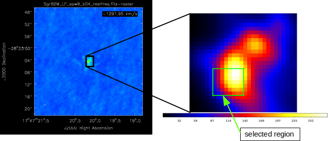
Fig. 17 The selected region, we want to describe.
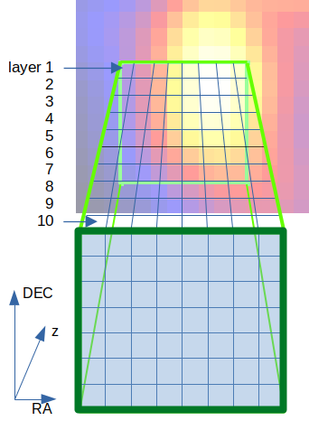
Fig. 18 Here, we use ten cells (layers) along the line of sight.
We start with selecting pixels we want to describe, where the spatial resolution of the used data files defines the spatial resolution within the RA-DEC plane, see Fig. 17. We are free to define the number of grid cells along the line of sight. Here, we use ten cells, see Fig. 18. Furthermore, we can set the center of the coordinate system arbitrarily. For many applications it is recommended to set the center of the coordinate system to the center of a specific grid cell.
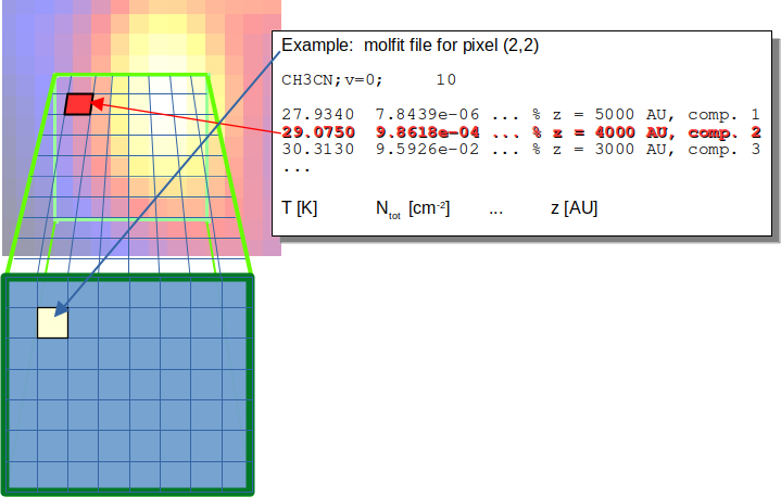
Fig. 19 Each cell along the line of sight is described by a component in the corresponding molfit file.
For each pixel within the RA-DEC plane, we have to create a molfit file, which describes components at ten different layers. Please note, that the component located at the layer close to the background must have the highest ordering parameter, as described in Sect. “Stacking”. The ordering parameter of each component is used to define the order of components along the line of sight. The exact value of the order parameter is irrelevant. One possible quantity can be the distance of each component to the observer. The number of molecules, RRLs or continuum contributions is not limited, but if more than one contribution (molecules, RRLs or continuum contributions) is defined for a given distance, the local overlap should be taken into account to correctly treat the different contributions within that cell. As the computational effort scales with the number of layers, the components describing the different contributions should be located at one of the (here ten) layers.
If e.g. the temperature is given by an analytic expression, the temperature for a given cell should be computed at the cell center. Note that if the density of a molecule is given by an analytical expression, the column density must be calculated by integrating the density of the cell along the line of sight.